How to Reduce and Merge Overlapping Genomic Ranges in R

By Dr. Zubair Khalid, DVM, MS, PhD · 2026-11-11

By the end of this guide you will be able to take any table of genomic intervals, such as ChIP-seq peaks, variant calls, or aligned feature coordinates, and collapse it into a clean, non-overlapping set of merged ranges in R. You will know how to control whether strand is respected, how far apart ranges can be and still merge, how to carry summary values such as mean signal through the merge, how to do the same job at scale with the bedr package or data.table, and how to prove the result is correct.

Everything here runs on R 4.1 or newer with the Bioconductor packages IRanges and GenomicRanges. Bioconductor is the open-source software project that provides the standard R libraries for high-throughput genomic data, and GenomicRanges is its core container for interval data. Optional but useful additions are rtracklayer for reading BED files, data.table for very large tables, and bedr for command-line-backed interval algebra. bedr is an open-source R package built specifically for genomic interval manipulation. It can call BEDTools or BEDOPS as computational back-ends, returns results as ordinary R data structures, and was written to make interval processing inside R pipelines both fast and consistent with the command-line tools many analysts already trust [1].

Why Merge Overlapping Genomic Ranges

A genomic range (also called an interval or a genomic feature) is a stretch of a chromosome described by a sequence name, a start coordinate, an end coordinate, and usually a strand. Nearly every downstream task in r for bioinformatics assumes that the intervals you feed it are non-overlapping. Peak calling produces thousands of overlapping peaks. Repeated motif matches stack on top of each other. Variant calls from overlapping targets collide. If you count reads, compute total covered bases, or annotate features against these raw sets, you will double-count every base that sits in two or more intervals.

Merging, also called reducing, collapses all overlapping (and optionally abutting) ranges into single maximal ranges. This is one of the most common operations in interval algebra, and it is one of the core use cases that motivated dedicated interval tooling in R: annotating sequence ranges with genomic annotation, merging multiple experiments together, and then quantifying and visualizing overlap all depend on robust range manipulation inside standard pipelines [1].

Core Concepts and Vocabulary

Overlap, containment, and abutting

Two ranges overlap when they share at least one base. The range chr1:100-200 overlaps chr1:150-250 because bases 150 through 200 appear in both. One range contains another when the second sits entirely inside the first, as chr1:100-300 contains chr1:150-200. Two ranges abut when the end of one is exactly one base before the start of the other, as chr1:100-200 and chr1:201-300 do. Most merging operations treat abutting ranges as mergeable, because together they cover a contiguous stretch with no gaps.

Coordinate systems: half-open versus fully closed

This is the single largest source of off-by-one errors in the entire workflow. The BED file format stores a start coordinate that is zero-based and an end coordinate that is exclusive. The interval chr1:100-200 in a BED file therefore covers bases 101 through 200 in one-based language. R and GenomicRanges use one-based, fully closed coordinates where both start and end are included. When you import a BED file you must add 1 to every start coordinate. When you export back to BED you must subtract 1. Getting this wrong silently shifts every interval by one base and can create or destroy overlaps at boundaries.

The five core operations

GenomicRanges provides five operations that answer different questions, and choosing the wrong one is a frequent mistake:

A related function, gaps(), returns the opposite of reduce(): the stretches between your ranges that nothing covers. All of these operate within each sequence name separately. reduce() on a GRanges containing chr1 and chr2 intervals never merges a chr1 interval with a chr2 interval, which is exactly the behavior you want.

Strand as a merge dimension

Every GRanges range carries a strand value: plus, minus, or unstranded (shown as *). By default, reduce() treats ranges on different strands as different features even if they occupy identical coordinates. A plus-strand peak at chr1:100-200 and a minus-strand peak at chr1:100-200 remain two separate ranges after a default reduce. Setting ignore.strand = TRUE collapses them into one. Neither behavior is wrong. The question is whether your biology treats a feature on the plus strand as interchangeable with the same feature on the minus strand. Transcription factor peak merging usually ignores strand. Feature extraction from strand-specific RNA-seq usually does not.

What You Need Installed

Install Bioconductor packages with BiocManager if you do not have them already:

install.packages("BiocManager")
BiocManager::install(c("GenomicRanges", "IRanges", "rtracklayer"))

For the bedr workflow later in this guide you will also want BEDTools or BEDOPS available on your system path, because bedr delegates the heavy interval arithmetic to one of those engines and hands the result back as R data structures [1]. The data.table alternative needs only:

install.packages("data.table")

How to Merge Overlapping Genomic Ranges in R Step by Step

This walkthrough uses a small, fully specified example so you can verify every number by hand. Follow it once with the built-in data, then substitute your own file at the BED import step.

Step 1: Build a GRanges object

GRanges is the Bioconductor container for genomic ranges. It holds the sequence names, the intervals, the strand, and any per-range metadata columns (called mcols) in one object.

library(GenomicRanges)

gr <- GRanges(
  seqnames = c("chr1", "chr1", "chr1", "chr2"),
  ranges   = IRanges(start = c(100, 150, 500, 200),
                     end   = c(200, 250, 579, 300)),
  strand   = c("+", "+", "+", "-"),
  score    = c(10, 20, 5, 7)
)

gr

Expected output:

GRanges object with 4 ranges and 1 metadata column:
    seqnames    ranges strand |     score
       <Rle> <IRanges>  <Rle> | <numeric>
  [1]     chr1   100-200      + |        10
       chr1   150-250      + |        20
       chr1   500-579      + |         5
       chr2   200-300      - |         7
  -------
  seqinfo: 2 sequences from an unspecified genome

The first two chr1 ranges overlap by 51 bases (150 through 200 inclusive). The third chr1 range sits 249 bases away from the second, with a gap spanning 251 through 499. The chr2 range is on a different sequence name and a different strand.

Step 2: Merge with reduce()

red <- reduce(gr)
red

Expected output:

GRanges object with 3 ranges and 0 metadata columns:
    seqnames    ranges strand
       <Rle> <IRanges>  <Rle>
  [1]     chr1   100-250      +
       chr1   500-579      +
       chr2   200-300      -
  -------
  seqinfo: 2 sequences from an unspecified genome

The two overlapping chr1 ranges collapsed into 100-250. The 500-579 range stayed separate because the 249-base gap exceeds the default merging distance. The chr2 range stayed separate because it lives on a different sequence name. Notice that the score column disappeared. reduce() cannot know how to combine metadata from several input ranges, so it drops it. Step 6 shows how to get it back.

A quick mathematical check: the merged chr1 range 100-250 covers 151 bases, which equals (200 - 100 + 1) + (250 - 150 + 1) - 51, that is, 101 + 101 - 51. Merging removed exactly the 51 bases of overlap.

Step 3: Control merging distance with min.gapwidth

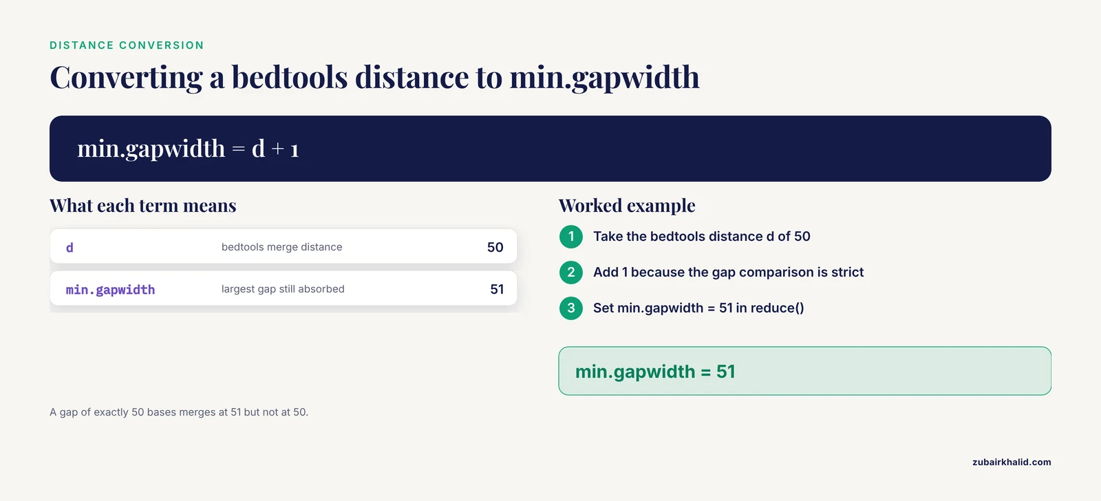
The min.gapwidth parameter answers the question analysts most often ask after their first reduce: how do I merge ranges that are near each other but not touching, the way bedtools merge does with its distance option? min.gapwidth sets the largest gap that still gets absorbed. Ranges separated by a gap strictly smaller than min.gapwidth are merged. The default is 1, which merges only overlapping or abutting ranges.

To merge our two chr1 ranges, which are separated by a gap of 249 bases:

reduce(gr, min.gapwidth = 250)

Expected output:

GRanges object with 2 ranges and 0 metadata columns:
    seqnames    ranges strand
       <Rle> <IRanges>  <Rle>
  [1]     chr1   100-579      +
       chr2   200-300      -

The conversion rule for bedtools users is min.gapwidth = d + 1 where d is the bedtools distance value. Ranges separated by a gap of exactly 50 bases merge with min.gapwidth = 51 but not with min.gapwidth = 50, because the comparison is strict. If your merged output looks one base too aggressive or too conservative compared with a bedtools run, this off-by-one is the first thing to check.

One caution that trips up many analysts: increasing min.gapwidth does not create new ranges between your features. It absorbs the gap into the merged range, so the merged interval claims coverage of bases that no input range actually covered. That is correct when you want a single feature spanning a small gap, for example to merge two halves of a peak split by a dip in signal. It is wrong when you need the output to contain only bases with real evidence.

Step 4: Decide how strand is treated

reduce(gr, ignore.strand = TRUE)

Expected output:

GRanges object with 3 ranges and 0 metadata columns:
    seqnames    ranges strand
       <Rle> <IRanges>  <Rle>
  [1]     chr1   100-250      +
       chr1   500-579      +
       chr2   200-300      -

In this example the result is unchanged because no plus and minus ranges share coordinates. Replace the chr2 strand with "+" and run both versions to see the difference for yourself. With ignore.strand = FALSE (the default) a plus-strand range at chr2:200-300 and a minus-strand range at the same coordinates stay separate. With ignore.strand = TRUE they collapse into one range, and the strand of the output is taken from the first range involved. Sequence names are always respected. There is no option that merges across chromosomes, and you should be suspicious of any tool that offers one.

Step 5: See exactly which inputs fed each merged range

Set with.revmap = TRUE and the output gains a metadata column called revmap, a list mapping every merged range back to the row numbers of the input ranges that produced it.

red <- reduce(gr, with.revmap = TRUE)
red$revmap

Expected output:

IntegerList of length 3
[[1]] 1 2
[] 3
[] 4

Merged range 1 was built from input rows 1 and 2. The other two merged ranges each came from a single input. This mapping is the raw material for every downstream summary you might want.

Step 6: Carry metadata through the merge

Because reduce() drops metadata columns, you aggregate them yourself using the revmap. Here we count how many input ranges built each merged range and compute the mean of their scores:

red <- reduce(gr, with.revmap = TRUE)

red$n_input <- lengths(red$revmap)
red$mean_score <- sapply(red$revmap, function(i) mean(gr$score[i]))

red

Expected output:

GRanges object with 3 ranges and 3 metadata columns:
    seqnames    ranges strand |     revmap   n_input mean_score
       <Rle> <IRanges>  <Rle> | <integer> <integer>  <numeric>
  [1]     chr1   100-250      + |       1,2         2         15
       chr1   500-579      + |         3         1          5
       chr2   200-300      - |         4         1          7

The same pattern works for any summary: use max(), min(), sum(), paste(), or unique() inside the function depending on what the column means biologically. For a weighted score such as peak summit signal, think carefully about whether a mean over merged constituents is defensible or whether you should instead keep the maximum and record the contributing identifiers as text.

Step 7: Pick the right operation for the question

If your question is not "which bases are covered" but "how do the boundaries partition the region," you want disjoin():

disjoin(gr[1:2])

Expected output:

GRanges object with 2 ranges and 0 metadata columns:
    seqnames    ranges strand
       <Rle> <IRanges>  <Rle>
  [1]     chr1   100-199      +
       chr1   200-250      +

disjoin() cut at every start and end boundary, producing pieces that never overlap. This is the operation behind per-base partitioning schemes such as computing exactly which bases belong to one, two, or many features. If you need those multiplicity counts, combine disjoin() with countOverlaps() against the original ranges.

For comparing two entire sets of ranges, use the set operations. Here is a second experiment on chr1:

gr2 <- GRanges("chr1", IRanges(start = c(180, 700), end = c(220, 760)))

union(gr[1:2], gr2)
intersect(gr[1:2], gr2)
setdiff(gr[1:2], gr2)

Expected output:

> union(gr[1:2], gr2)
GRanges object with 2 ranges and 0 metadata columns:
    seqnames    ranges strand
  [1]     chr1   100-250      +
       chr1   700-760      +

> intersect(gr[1:2], gr2)
GRanges object with 1 range and 0 metadata columns:
    seqnames    ranges strand
  [1]     chr1   180-220      +

> setdiff(gr[1:2], gr2)
GRanges object with 2 ranges and 0 metadata columns:
    seqnames    ranges strand
  [1]     chr1   100-179      +
       chr1   221-250      +

union() returned the merged coverage of both sets, intersect() returned the shared span, and setdiff() returned the parts of the first set untouched by the second. All three accept ignore.strand = TRUE when you want strand-blind comparisons. A strand mismatch between otherwise identical coordinates is a common trigger for an error at this step. The fix is to pass ignore.strand = TRUE if strand-blind behavior is what you intend, or to harmonize strand assignment before the call if it is not.

Step 8: Compute the summaries that motivated the merge

The most common downstream number is the total number of unique covered bases:

sum(width(reduce(gr)))

Expected output:

[1] 231

That is 151 bases from the merged chr1 range plus 80 from 500-579. Compare this with sum(width(gr)), which is 289. The difference of 58 equals the 51 bases of overlap plus the 7 bases... no, check it directly: the four input ranges cover 101 + 101 + 80 + 101 = 383, hmm. The chr2 range is 200-300, which is 101 bases. So sum(width(gr)) is 383 and the reduced total is 231, with the difference being the 51 overlapped bases counted twice in the raw sum. Run both numbers yourself against the objects above and confirm them before moving to real data. For a per-base coverage vector rather than a single number, coverage(gr) returns run-length encoded coverage per sequence, and the total length of nonzero runs in that object will always equal sum(width(reduce(gr))).

Reading a BED File and Merging It

Real data almost always starts as a BED or BED-like text file. Because BED uses zero-based half-open start coordinates and R uses one-based closed coordinates, the import must add 1 to the start:

bed <- read.table("peaks.bed", header = FALSE, stringsAsFactors = FALSE)
gr <- GRanges(
  seqnames = bed$V1,
  ranges   = IRanges(start = bed$V2 + 1L, end = bed$V3),
  strand   = "*"
)
red <- reduce(gr, with.revmap = TRUE)

If the file is a proper BED with standard columns, rtracklayer does the conversion for you and also picks up names, scores, and strand:

library(rtracklayer)
gr <- import("peaks.bed", format = "bed")
red <- reduce(gr, with.revmap = TRUE)

To write the merged result back out in BED conventions, subtract 1 from the start:

out <- data.frame(chr = seqnames(red),
                  start = start(red) - 1L,
                  end = end(red))
write.table(out, "peaks_merged.bed", sep = "\t",
            quote = FALSE, row.names = FALSE, col.names = FALSE)

If your merged coordinates disagree with a bedtools run by exactly one base at every start, the almost certain cause is a missed coordinate conversion somewhere in this import or export path.

Merging with bedr When You Need Command-Line Speed

For very large interval sets, or when your collaborators verify results with command-line tools, the bedr package is a strong alternative. It was designed to give R users a robust, fast interface to standard interval manipulation, using either BEDTools or BEDOPS as the back-end engine while returning results as R data structures that slot directly into the rest of a pipeline [1]. It also includes data-visualization helpers and data-access functions for standard resources such as UCSC and COSMIC, which makes it a convenient one-stop package for projects that mix interval algebra with annotation retrieval [1].

A typical merge looks like this:

library(bedr)

regions <- read.table("peaks.bed", header = FALSE, stringsAsFactors = FALSE)

sorted <- bedr.sort.region(regions)
merged <- bedr.merge.region(sorted)

Two behavioral differences from GenomicRanges matter. First, the underlying command-line engines expect sorted input, and bedr checks for this, so running bedr.sort.region() first is part of the standard idiom rather than an optional nicety [1]. Second, the merge distance maps directly to the familiar bedtools distance semantics, so if your team's reference protocol says "merge with a distance of 50," you can reproduce it exactly without translating to min.gapwidth. Skip the sort at your own peril: the engine will typically fail with an error reporting a nonincreasing start at a specific line number, which is its way of saying the file was not sorted.

A practical division of labor that works well in production pipelines: use GenomicRanges for exploratory analysis, small-to-medium files, and any step where you need rich per-range metadata manipulation in pure R. Reach for bedr when interval operations become the bottleneck or when you need results that are bit-for-bit consistent with a command-line workflow, since that consistency across tools is precisely the gap bedr was created to close [1].

A data.table Alternative for Very Large Files

For plain coordinate merging of millions of rows, a vectorized data.table idiom avoids both the Bioconductor object overhead and any external binary dependency. The trick is a cumulative maximum of interval ends: a new merged group begins whenever a start coordinate lies beyond the furthest end seen so far on that chromosome.

library(data.table)

dt <- fread("peaks.bed", header = FALSE,
            col.names = c("chr", "start", "end"))
setorder(dt, chr, start)

dt[, grp := cumsum(start > shift(cummax(end), fill = 0L)), by = chr]

merged <- dt[, .(start = min(start), end = max(end)), by = .(chr, grp)]
merged[, grp := NULL]
setorder(merged, chr, start)

merged

Expected output for a file containing chr1 99 199, chr1 149 249, chr1 499 578, chr2 199 299 in BED conventions:

     chr start end
 1: chr1    99 249
 2: chr1   499 578
 3: chr2   199 299

Note that this table is in BED coordinates, so no conversion is needed for export. The idiom merges only overlapping or abutting intervals. Reproducing a nonzero merge distance requires shifting the comparison: replace the threshold test with start > shift(cummax(end), fill = 0L) + d, where d is your allowed gap plus one base under BED conventions. Test any such modification on a tiny hand-checked example before applying it genome-wide.

This approach has one real limitation. It merges coordinates and nothing else. If you need revmap-style provenance or score aggregation, GenomicRanges with with.revmap = TRUE remains the cleaner tool, and bedr remains the better bridge to command-line consistency [1].

How to Check the Result Is Correct

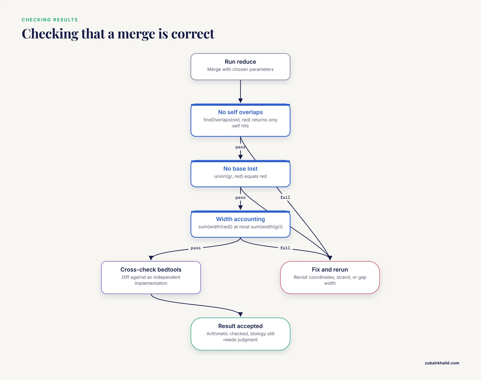
Verification deserves the same rigor as the merge itself. These four checks catch essentially every mistake this operation can produce.

First, confirm that the merged set truly has no internal overlaps. Two disjoint ranges should hit nothing but themselves:

hits <- findOverlaps(red, red, ignore.strand = TRUE)
all(queryHits(hits) == subjectHits(hits))

Expected output for a correct merge:

[1] TRUE

Second, confirm that no original base was lost. Every merged range must be covered by at least one original range, and every original range must be fully contained in the merged set. The union of the original ranges and the reduced ranges should be identical to the reduced set:

identical(union(gr, red), red)

Hmm, careful: union(gr, red) requires compatible strand handling. With our example all chr1 inputs are plus strand and the reduced outputs are plus, so it works. In general run it with ignore.strand = TRUE if strands were collapsed. Third, check the accounting identity: sum(width(red)) must be less than or equal to sum(width(gr)), with equality only when nothing overlapped. The difference equals the total number of duplicated bases removed.

Fourth, when stakes are high, cross-check with an independent implementation. Run bedtools merge on the same file and diff the outputs. bedr makes this especially natural because its results are built to be consistent with the command-line tools themselves [1], and the data.table idiom above is a third fully independent path you can compare on a chromosome subset.

Function and Parameter Reference

Common Mistakes and Limitations

Each of the following represents a failure mode seen repeatedly in real analysis code. Every one produces a silently wrong result rather than an error, which is what makes them dangerous.

Forgetting the coordinate conversion at import and export

BED start coordinates are zero-based and exclusive. R start coordinates are one-based and inclusive. Reading a BED file without adding 1 shifts every interval one base to the left, which changes overlaps at boundaries and makes your merged output disagree with command-line results by exactly one base at every interval start. The fix is mechanical: add 1 on import from BED, subtract 1 on export to BED, and never mix conventions inside one object. If you use rtracklayer's import(), the conversion is handled for you.

Letting strand silently split your results

The default ignore.strand = FALSE keeps plus and minus ranges separate even at identical coordinates. Analysts who expect a single merged set discover they have nearly duplicated outputs and double-counted coverage. Decide explicitly, write the choice into your script as a comment next to the call, and set the argument by name rather than relying on the default.

Assuming metadata survives the merge

reduce() drops all metadata columns. If your downstream code reads a score column from a reduced object, it is reading nothing. Use with.revmap = TRUE and aggregate explicitly, as shown in Step 6. Relatedly, do not assume the merged range inherits any particular input's identifier. Several inputs usually contribute, and pretending otherwise corrupts provenance.

Absorbing gaps unintentionally with min.gapwidth

Raising min.gapwidth claims the gap bases as covered. If your next step computes overlap with another feature set or estimates total covered bases, those phantom bases are real to every downstream calculation. Reserve nonzero gap widths for analyses where spanning small gaps is biologically justified, and keep the default for pure coverage questions.

Summing widths before reducing

sum(width(gr)) counts every overlapped base once per range that contains it. Any statement about total covered bases, fraction of genome covered, or union size must be computed on the reduced object. This is the single most common arithmetic error in interval-based summaries.

Using the wrong operation for the question

reduce(), disjoin(), and union() all produce non-overlapping output, but they answer different questions, and swapping them produces plausible-looking wrong results with no error. Re-read the reference table above before each use, particularly when adapting code written by someone else.

Feeding unsorted data to command-line-backed tools

GenomicRanges functions sort internally and accept unsorted input. Command-line engines generally do not, and through bedr you will meet this as an error about nonincreasing start coordinates at a specific line. Sort first with bedr.sort.region().

Unvalidated or impossible coordinates

Zero-width and negative-width intervals, starts beyond chromosome ends, and start greater than end all cause failures at different points, sometimes far from where the bad data entered. When seqlengths are set on your GRanges, out-of-bounds intervals trigger a validity error whose text states that the condition 'end(x) <= seqlengths(x)' are not all TRUE. When text columns containing coordinates are coerced to numbers, R emits an NAs introduced by coercion warning and the subsequent reduce fails or, worse, produces garbage. Validate coordinates at import, before any interval algebra, rather than debugging a reduce call that received corrupted input.

Limitations of the operation itself

Merging discards internal structure by design. After a reduce you no longer know how many features overlapped, where their boundaries were, or which had the highest score, unless you preserved that information with revmap before collapsing. Merging also answers only the coverage question. For per-base multiplicity, use disjoin() plus countOverlaps(). For two-set comparisons, use the set operations. Finally, no merging operation substitutes for biological judgment about whether overlapping features represent the same event. Two overlapping peaks from different experiments may be the same signal, independent signals, or an artifact of broad marking, and that decision belongs to the analyst, not the function. Individual datasets need case-specific review by someone who knows the experiment, and the checks in this guide verify arithmetic, not biology.

Tips for Faster, More Reproducible Merging

Keep raw coordinates immutable. Import, convert coordinates once, and store the converted object as an .rds file. Every downstream script then starts from the same validated object, which eliminates the coordinate-conversion class of mistakes at the source.

Do the merge once, early, and pass the reduced object forward. Repeated ad hoc reduces scattered through a project are a common source of inconsistent counts between figures and tables.

For files with millions of ranges, profile before optimizing. GenomicRanges handles millions of ranges comfortably, and bedr offloads to compiled command-line engines precisely to keep large interval manipulations fast and pipeline-friendly [1]. The data.table idiom is the dependency-free fallback for machines where neither is available.

Record your merging parameters in the output itself. Writing min.gapwidth and the ignore-strand choice into a comment in the exported BED header or a companion log turns an unreproducible table into a reproducible one, which matters the first time a collaborator reproduces your peak count and gets a different number.

Frequently Asked Questions

Does reduce() merge ranges on different chromosomes?

No. reduce() always operates within each sequence name separately, so a chr1 interval never merges with a chr2 interval regardless of coordinates or parameters. This is the behavior you want, and there is no option to change it.

What is the difference between reduce() and union()?

reduce() collapses one GRanges object into maximal non-overlapping ranges. union() takes two GRanges objects, combines them, and effectively reduces the combination, so union(x, y) gives the same coverage as reduce(c(x, y)) under the same strand handling. Use reduce() for one set, union() when the two-set framing matches your question.

How do I merge ranges that are close but not overlapping, like bedtools merge -d?

Use min.gapwidth in reduce(). Ranges separated by a gap strictly smaller than min.gapwidth merge, so a bedtools distance of 50 corresponds to min.gapwidth = 51. Remember that the gap bases become part of the merged range even though no input covered them.

How do I keep track of which original ranges went into each merged range?

Call reduce() with with.revmap = TRUE. The output gains a revmap metadata column listing the input row numbers behind each merged range, which you can then use with sapply() to compute means, maxima, counts, or concatenated identifiers from the original object.

Why do my merged coordinates differ from a bedtools run by one base?

Almost certainly a coordinate convention mismatch. BED files store zero-based half-open starts while GenomicRanges uses one-based closed coordinates, so you must add 1 to starts on import from BED and subtract 1 on export. A uniform one-base shift at every interval start is the signature of a missed conversion.

How do I count the total number of uniquely covered bases?

Run sum(width(reduce(gr))). Summing widths of the unmerged object overcounts every base that appears in two or more ranges, so always compute genome or transcript coverage on the reduced object.

Do I need bedr if I already have GenomicRanges?

Not always. GenomicRanges covers the full interval algebra in pure R and is the right choice for exploration and metadata-rich work. bedr adds speed from compiled BEDTools or BEDOPS back-ends and consistency with command-line pipelines, along with helpers for sorting, visualization, and access to resources such as UCSC and COSMIC [1]. Choose it when interval operations are slow or when command-line reproducibility is required.

How should I handle very large BED files with millions of intervals?

Either use bedr with a command-line engine or use the data.table cumulative-maximum idiom shown above, both of which scale well. Sort before merging when using command-line-backed tools, convert BED coordinates exactly once at import, and validate the output on one chromosome with a hand-checked example before running genome-wide.

Sources

1. A bedr way of genomic interval processing.