Matplotlib vs. Seaborn for Biological Data Visualization
By Dr. Zubair Khalid, DVM, MS, PhD ·

Matplotlib is a general-purpose drawing library that gives you pixel-level control over every element of a figure, while Seaborn is a statistical plotting layer built on top of matplotlib that turns tidy DataFrames into polished distribution, relationship, and categorical plots with one line of code. The rule of thumb for bioinformatics work is simple: use Seaborn when you are exploring a DataFrame of samples, features, and groups, and use matplotlib when you need a custom scientific graphic, a multi-panel publication figure, or exact control over coordinates, axes, and annotations. Most experienced analysts use both in the same notebook, because Seaborn returns matplotlib objects and everything Seaborn draws can be edited with matplotlib commands.
This article walks through the real difference between matplotlib and seaborn for bioinformatics, the decision criteria that matter in day-to-day analysis work, and worked scenarios drawn from published biological visualization workflows, including protein structure data, elemental imaging, sequence design evaluation, GWAS pipelines, and mass spectrometry imaging. If you are learning python for bioinformatics, understanding how these two libraries divide the work is one of the highest-leverage things you can do early, because it saves you from fighting the wrong tool for the job.
The Short Answer for Working Bioinformaticians
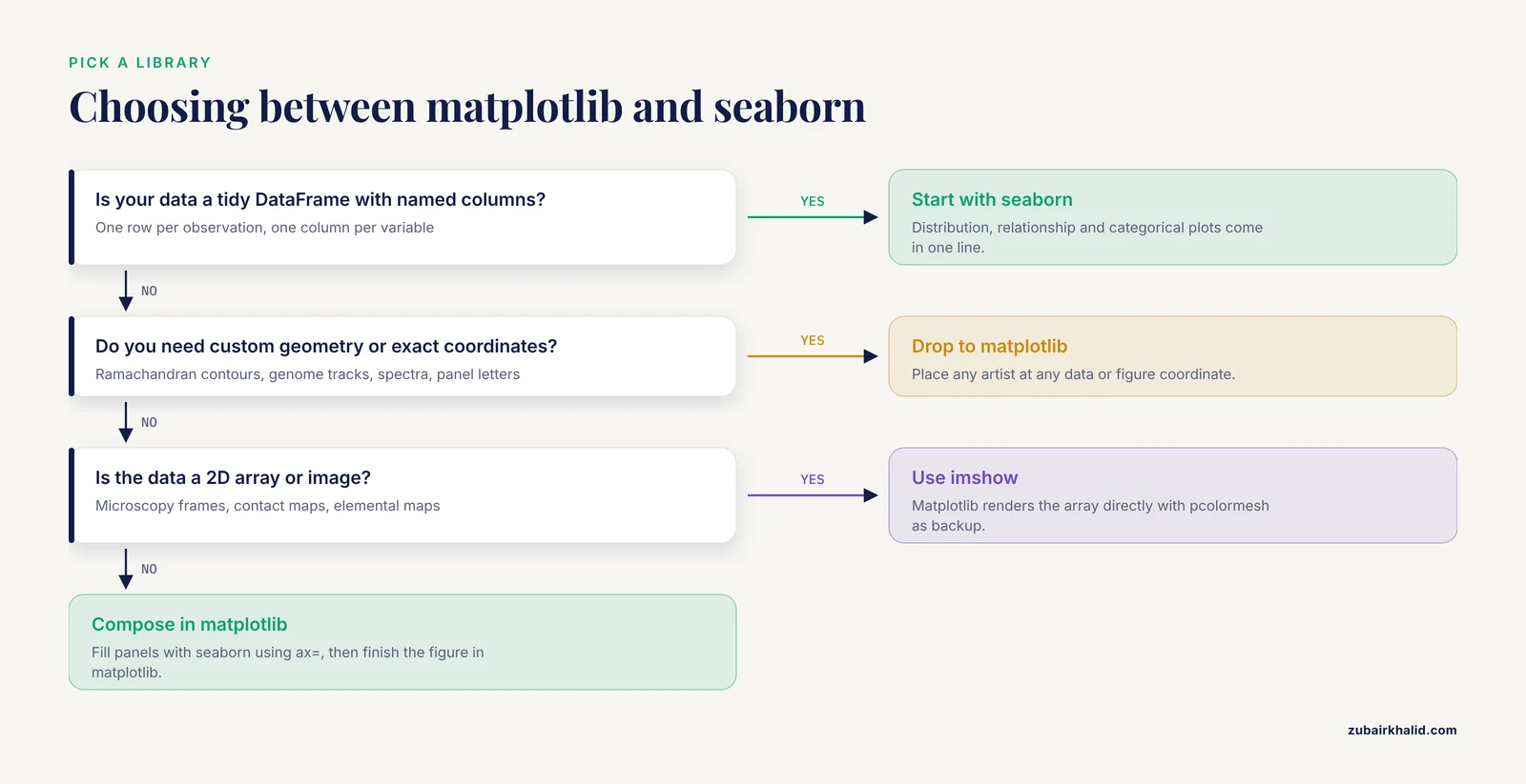
The difference between matplotlib and seaborn is a difference in abstraction level. Matplotlib exposes a figure object model where you place axes, set coordinate systems, and draw primitives such as lines, markers, polygons, text, and images. Seaborn starts one level higher. You hand it a DataFrame in tidy format (one row per observation, one column per variable), name the columns you want on each axis, and Seaborn handles grouping, aggregation, statistical estimation, color mapping, and legend construction for you.
A useful way to remember it: Seaborn answers questions, matplotlib draws answers. When you are still asking what your RNA-seq count table or mass spectrometry feature table looks like, Seaborn gets you a distribution plot, a pairwise scatter matrix, or a clustered heatmap in seconds. When you know exactly what the figure must show, for example a Ramachandran plot with reference contours and labeled regions of allowed backbone dihedral angles, matplotlib's lower-level control is what makes the figure possible at all.
The published bioinformatics literature uses both, usually together. A workshop on exploring large volumes of protein data from the Protein Data Bank taught participants to load structures with Python and visualize trends in amino acid abundance, backbone dihedral angles, and secondary structure using both matplotlib and seaborn in Jupyter notebooks [1]. That pairing, one library for the statistical overview and one for the custom scientific graphic, is the normal pattern across the field.
What Matplotlib Is, and Where It Fits in Python for Bioinformatics
Matplotlib is the foundational plotting library of the scientific Python ecosystem. It has been the default plotting backend for NumPy, SciPy, pandas, and scikit-learn for most of two decades, which means nearly every bioinformatics package that produces a plot in Python eventually calls matplotlib underneath, whether or not you see it.
The object model, in plain terms
Three concepts cover most of what you need:
- Figure. The whole canvas, the thing that gets saved to PDF or PNG.
- Axes. One plotting region inside the figure with its own x axis, y axis, title, and ticks. A figure can hold many Axes, which is how multi-panel figures are built.
- Artists. The individual drawn things, including Line2D objects, collections of markers, text labels, spans, arrows, and images.
This hierarchy is why matplotlib dominates when the figure geometry is unusual. A scatter plot of phi versus psi backbone dihedral angles with shaded regions for alpha-helical and beta-strand conformations, a multiple sequence alignment rendered as a colored grid with residue annotations, or a genome track diagram with arrows for genes are all straightforward in matplotlib because you can place any drawing primitive at any data or figure coordinate. The protein visualization workshop mentioned above uses exactly this approach, walking students through Python functions, data loading, and custom plots of protein structural trends in Jupyter notebooks [1].
What matplotlib buys you in a biology workflow
- Exact axes and coordinate control. You can place an inset, break an axis, draw a secondary x axis in a different unit (for example base pairs on top and kilobases below), and annotate data points with leader lines.
- Image display.
ax.imshow()renders a 2D array directly. This covers microscopy frames, gel-like heatmaps, contact maps from chromatin conformation capture, and pixel grids from imaging mass spectrometry. - Multipanel composition.
plt.subplots()andGridSpeclet you build a Figure 3 with panels A through F of mixed types, shared axes, and precise spacing. - Deterministic output. The same script produces the same PDF, which matters when a journal asks for a revision with one changed font size three months later.
What Seaborn Is, and Why It Spread Through Biology Labs
Seaborn is a data visualization library built on matplotlib with two design goals. First, statistical graphics should be one-liners. Second, plotting functions should accept tidy DataFrames natively, so the structure of your data (which pandas encourages, and which BioPythony and scikit-learn pipelines produce) maps directly onto the structure of the plot.
The statistical graphics layer
Seaborn groups its functions into three families that map cleanly onto biological questions:
- Relational plots (
scatterplot,lineplot) for relationships between continuous variables, for example expression of a gene across a time course with confidence intervals computed automatically from replicate spread. - Distribution plots (
histplot,kdeplot,boxplot,violinplot,ecdfplot) for comparing groups, which covers the majority of quality control in omics workflows. - Categorical and matrix plots (
barplot,countplot,pointplot,heatmap,clustermap) for enrichment results, sample-by-sample correlation matrices, and clustered expression heatmaps.
The key behavior is statistical estimation. lineplot with multiple observations per x value draws the mean line and a bootstrap confidence band by default. boxplot and violinplot split data by one or two categorical variables without you writing a groupby call. For exploratory analysis of a phenotype table, a metadata sheet, or a differential expression result, this removes most of the boilerplate.
Styling as a default, not a chore
sns.set_theme() applies a coherent set of colors, grid, and font scales that looks reasonable out of the box. The colorblind-friendly palettes matter in biology publishing, where reviewers increasingly expect figures readable under color vision deficiency, and Seaborn makes switching palettes a one-line change.
Side-by-Side Comparison Table
The table below is the core of the matplotlib vs. seaborn decision for biological data visualization. Every row reflects how the two libraries behave in real analysis sessions.
| Dimension | matplotlib | Seaborn |
|---|---|---|
| Abstraction level | Low-level figure and axes object model | High-level statistical plot functions |
| Relationship | The foundation layer | Built on matplotlib, returns matplotlib objects |
| Native input | Arrays, lists, and coordinates you compute yourself | Tidy pandas DataFrames with named columns |
| Grouping by category | Manual (loop over groups, assign colors yourself) | Automatic (map a categorical column to hue, style, and markers) |
| Statistical summaries | You compute them (mean, CI, regression) and draw the result | Built in (confidence bands, box statistics, regression fits, bootstrapping) |
| Custom scientific graphics | Strength (Ramachandran plots, track diagrams, spectra, image panels) | Weak (possible but awkward to force) |
| Exploratory speed on a new DataFrame | Slower, more code per plot | Very fast, often one line per question |
| Multipanel publication figures | Strength (subplots, GridSpec, shared axes, panel labels) | Supports it via ax= arguments and figure-level functions, less flexible |
| Theming and palettes | Manual rcParams configuration | set_theme() plus curated palettes in one line |
| Legend and colorbar handling | Manual placement and labeling | Automatic, usually correct on first try |
| Performance on huge point clouds | Better, with rasterization, hexbin, and raw array rendering | Same ceiling, since it calls matplotlib, but defaults encourage dense overplotted scatters |
| Learning curve | Steeper, more concepts (Figure, Axes, transform, artist) | Gentle for standard plots, confusing once you need nonstandard geometry |
| Typical bioinformatics role | Final publication figures, custom structural and genomic graphics | Exploration, QC, group comparisons, clustered heatmaps |
One clarification that prevents a common confusion in the "matplotlib or seaborn" debate: choosing Seaborn is not choosing against matplotlib. Every Seaborn call creates a matplotlib Figure and Axes. When you call sns.boxplot(ax=ax), you can then adjust that Axes with matplotlib commands. The comparison is really about which entry point you start from.
When to Use Matplotlib
The case for reaching for matplotlib first comes down to four situations that appear constantly in biological data visualization.
1. Custom scientific plot types
Biology has a long tail of domain-specific graphics that no plotting library ships as a built-in. Ramachandran plots with contour lines marking allowed and generously allowed phi/psi regions. Dot plots and arc diagrams for structural RNA. Synteny ribbons between genomes. Spike raster plots for electrophysiology. Spectrum plots with stacked traces from replicate mass spectrometry runs. None of these are one call in any library, and Seaborn's DataFrame-centric API actively gets in the way when your data is a set of geometric coordinates rather than an observations-by-variables table.
The published record backs this pattern. A custom Python pipeline for GWAS fine-mapping used Python-coded scripts for genome-wide visualization, Manhattan-style signal rendering, and downstream systems biology plots as part of an end-to-end PTSD risk variant analysis [2]. That kind of genome-scale graphic, with chromosomes arranged along the x axis and significance thresholds drawn as reference lines, is classic matplotlib territory.
2. Rendering images and pixel data
Any time your data is fundamentally a 2D array of numbers, matplotlib's imshow and pcolormesh are the direct path. This includes:
- Microscopy and tissue imaging. The blender tissue cartography project, which maps curved epithelial surfaces from volumetric microscopy onto 2D projections, ships an accompanying Python library for quantitative analysis of the cartographic projections, and those projections are image data that Python plotting handles natively [3].
- Spatial elemental imaging. Laser ablation ICP-TOF-MS produces spatially resolved elemental channels where each pixel carries coordinates and intensities, and the ScaleBarOn and Muad'Data tools were built in Python to visualize and compare these element maps across specimens with consistent scaling [4].
- Contact maps, coverage tracks, and gel-like matrices from genomics.
Seaborn can display matrices through heatmap, but once you need nonuniform pixel sizes, log-scaled color, overlaid contours, or mixed image and vector content in one Axes, you are writing matplotlib anyway.
3. Publication-grade multipanel figures
Journals want figures with specific fonts, panel letters, shared legends, and controlled margins. Building those with plt.subplots(ncols=3, nrows=2, width_ratios=), then labeling panels A through F with ax.text() in figure coordinates, is the standard professional route. Seaborn contributes individual panels to such figures through the ax= parameter, but the composition logic lives in matplotlib.
4. Interactive or live monitoring displays
Matplotlib's animation API and fast redraw of line and image artists make it the rendering layer for dashboards and live monitors. At a synchrotron structural biology facility, the QuickProcess2 package uses a low-latency live image viewer as part of a Python-based system that unifies diffraction image visualization, automated processing, and experiment tracking for serial crystallography [5]. You would not build that kind of continuously updating display on Seaborn's figure-level functions.
When to Use Seaborn
Seaborn earns its place whenever the question is statistical and the data is already a table. These are the recurring situations.
1. Exploratory data analysis on a new dataset
The first hour with any new omics table follows the same script: distributions of each numeric column, counts per category, scatter plots of read depth versus GC content, pairwise relationships between metadata variables. Seaborn's histplot, countplot, scatterplot, and pairplot answer these in single calls, with hue mapping for your condition labels. In spectral clustering workflows for high-dimensional omics data, the PySimi framework pairs similarity matrix construction and clustering with downstream dimensionality reduction and visualization in a single consistent workflow [6], and that kind of dimensionality-reduction-plus-plot step is exactly where Seaborn's scatter and density functions get heavy use.
2. Group comparisons and replicate QC
Comparing expression of a gene across treatment groups, checking whether replicate correlations cluster by batch, verifying that normalized count distributions overlap across samples: these are boxplot, violinplot, and kdeplot questions. Seaborn draws them with correct grouping, ordering, and legends from column names alone.
3. Clustered heatmaps
sns.clustermap() performs hierarchical clustering on rows and columns and draws the dendrograms, matrix, and color annotations in one call. For a samples-by-genes matrix with a condition color annotation bar, this single function replaces roughly a hundred lines of manual scipy linkage code plus matplotlib bookkeeping. Sort-seq multiplexed assays of variant effect face a related visualization need, and the sortscore package provides convenient heatmap visualizations as a core feature of its Python scoring workflow for variant effect maps [7].
4. Regression and trend summaries
sns.regplot and sns.lmplot draw a scatter with a fitted line and confidence interval. For calibration curves in analytical work, dose-response previews, or correlation between two omics modalities, this is the fastest honest summary available. Mass spectrometry imaging pipelines make the same pairing of statistics and plot: the SPOT toolkit, implemented in both R and Python, integrates classification modeling, dimensionality reduction, and trajectory inference for spatially resolved proteomic profiles of breast disease progression [8], and each of those analytic outputs lands on a plot that a Python layer renders.
5. Visualization inside evaluation libraries
A clear trend in recent bioinformatics software is that authors build on the Python plotting stack rather than writing their own renderers, and Seaborn-style statistical graphics are the common vocabulary. The seqme library for evaluating biological sequence design from generative models includes diagnostics and visualization functions to inspect how designed sequences for peptides, DNA, mRNA, and proteins compare with target distributions [9]. The PhenoFECT package for plant phenology forecasting under climate change provides forecasting, exploration, and visualization across decades of open meteorological data, refining a chill-day model whose flowering predictions for three angiosperm species improved to a mean RMSE of 5.74 days [10]. In both cases the visualization layer exists because the underlying Python plotting libraries make adding it cheap.
Head-to-Head on the Criteria That Decide Real Choices
Time to first useful plot
Seaborn wins, usually by a wide margin. If your DataFrame has columns named sample, condition, and tpm, a publication-reasonable boxplot is sns.boxplot(data=df, x="condition", y="tpm"). The equivalent matplotlib code requires computing per-group statistics or plotting each group separately, setting colors, and building the legend by hand.
Final control over the finished figure
Matplotlib wins, and it is not close. Every property of every artist is settable: tick positions, fonts per text object, hatch patterns, path effects, custom projections, and exact figure dimensions. When a journal or thesis office imposes specific requirements, you satisfy them with matplotlib.
Fit to the shape of your data
This criterion decides most cases on its own. Tidy DataFrames with categorical columns favor Seaborn. Coordinate lists, images, matrices without an observation-per-row meaning, and geometry favor matplotlib. Much bioinformatics data sits in both camps at different pipeline stages. A single-cell dataset is a tidy cell-by-cell DataFrame for QC plots and a raw matrix for a heatmap, so a single notebook legitimately uses both.
Behavior at scale
Both libraries share the same rendering engine, so raw drawing speed is similar. The difference is in defaults and escape hatches. Matplotlib gives you rasterized=True for keeping huge point clouds out of your PDF file, hexbin and 2D histograms for overplotting, and direct array rendering. Seaborn's defaults happily draw half a million overlapping scatter points as a blob. The practical rule: for exploratory work on dense data, subsample or switch representation, and for anything rendered to vector output, set rasterization deliberately.
Reproducibility and provenance
Both are fully scriptable, which puts them ahead of point-and-click tools for reproducible python for bioinformatics workflows. The field's direction favors this strongly. Recent method papers emphasize reproducible, scripted execution across containerized pipelines, from a Nextflow workflow for small RNA-seq quantification that pairs its pipeline with a Streamlit application for interactive exploration and differential expression visualization [11], to an ATAC-seq pipeline that carries users from raw reads through quality control and genome accessibility analysis with explicit script-based steps [12], and an integrated ecosystem combining the ETE toolkit, TreeProfiler, and PhyloCloud for scalable annotation and visualization of large phylogenomic datasets [13]. Scripted plotting with matplotlib and Seaborn fits directly into that model, and pinning library versions in an environment file keeps figures stable across re-runs.
Relationship to the wider ecosystem
Specialized bioinformatics libraries are consumers of these two, not competitors. The ETE toolkit renders annotated phylogenetic trees through its own layout engine while remaining a Python package [13]. PhyloZoo provides data structures, algorithms, and dedicated visualization tools for phylogenetic networks in a unified Python framework [14]. The fast-nnt project reimplements neighbour-net algorithms for large phylogenetics with Python, R, and command line interfaces specifically so that network analysis becomes scriptable and reproducible on high-performance systems rather than locked inside GUI software [15]. When these libraries hand you data in Python, matplotlib and Seaborn are the general-purpose renderers you use for everything the specialized tool does not draw itself.
Worked Scenarios from Real Bioinformatics Workflows
Scenario 1: Teaching protein structure analysis with a Biopython tutorial
A workshop from the IUBMB/ASBMB Teaching Science with Big Data conference trained participants to explore large quantities of Protein Data Bank structures in Jupyter notebooks, using Python functions, Python-based data loading, and both matplotlib and seaborn to discover trends such as amino acid abundance, patterns in dihedral angles, and secondary structure frequencies, with all notebooks and data released openly under a CC BY-NC-SA 4.0 license at the BiopythonRamachandran repository [1]. The division of labor in that material is a model for a Biopython tutorial of your own. Seaborn handles the summary questions (histograms of residue frequencies, violin plots of dihedral angle distributions split by secondary structure class). Matplotlib handles the Ramachandran plot itself, where phi and psi angles need custom contour shading, degree-based axis ticks, and reference region outlines.
Scenario 2: Multi-specimen elemental imaging comparison
Elemental imaging by laser ablation ICP-TOF-MS yields several gigabytes of multi-channel pixel data per specimen, and comparing the same element across many specimens is central to interpretation in the life sciences. The ScaleBarOn and Muad'Data tools decompose multi-channel datasets into single-element matrix files in lightweight, widely supported formats so that scaled visualization and cross-specimen comparison become computationally tractable [4]. The design lesson generalizes: when data volume outgrows in-memory plotting, the pipeline splits rendering into per-element image tasks, which is a matplotlib-friendly pattern, while the exploration layer stays interactive.
Scenario 3: Benchmarking generative sequence designers
Evaluating computationally designed biological sequences requires comparing designed distributions against target distributions across sequence-based, embedding-based, and property-based metric groups, applicable to small molecules, DNA, ncRNA, mRNA, peptides, and proteins. The seqme library implements those metrics as a modular Python package with diagnostics and visualization functions, demonstrated on an antimicrobial peptide benchmark and on acquired mRNA data [9]. Distribution-overlap plots and metric scatter comparisons here are Seaborn-style jobs, while any per-sequence custom graphic drops down to matplotlib.
Scenario 4: GWAS fine-mapping and systems biology
A large-scale PTSD study built a custom Python pipeline spanning data harmonization from the GWAS Catalog, genome-wide visualization, linkage disequilibrium estimation against 1000 Genomes reference panels, approximate Bayesian fine-mapping, and haplotype inference, ultimately refining signals to 93 candidate SNPs across 66 genes from an initial set of 100 top-ranked SNPs [2]. Genome-wide visualization in such pipelines is a matplotlib composition problem: thousands of points along genomic coordinates, threshold lines, and annotation layers.
Scenario 5: Spectral clustering of omics data
PySimi unifies classical, adaptive, and neighborhood-based similarity measures for spectral clustering of bulk and single-cell RNA-seq data, with downstream dimensionality reduction and visualization plus an interactive web application for exploration, and showed that the similarity measure choice substantially changes clustering outcomes and biological interpretation [6]. The analytic takeaway for plotting is that embedding scatter plots (clusters in reduced space) are exploratory statements, Seaborn territory, and that their interpretation has limits addressed in the limitations section below.
Scenario 6: Forecasting and exploring phenology
PhenoFECT embeds 53 years of Korean meteorological data (1973 to 2025) for cherry, golden-bell, and azalea, refines chill-day model parameters against recent climate warming, and provides forecasting, exploration, and visualization across diverse open meteorological data [10]. Long-term climate series plotted with seasonal markers and per-species fits are a hybrid case: lineplot for the trends, matplotlib for the custom calendar and threshold annotations.
Scenario 7: Metabolomics processing with a GUI or code
Computational tools for LC-IMS-MS metabolomics from Pacific Northwest National Laboratory, including PNNL-PreProcessor, MZA, mzapy, LipidOz, PeakQC, and IonToolPack, provide both Python-based programmatic processing and GUI workflows so that researchers with different levels of computational experience can process, visualize, and interpret multidimensional mass spectrometry data reproducibly [16]. The dual-mode pattern matters: programmatic plotting (matplotlib and Seaborn) for pipelines, GUIs for discovery, and the same figure standards across both.
Combining Both Libraries in One Workflow
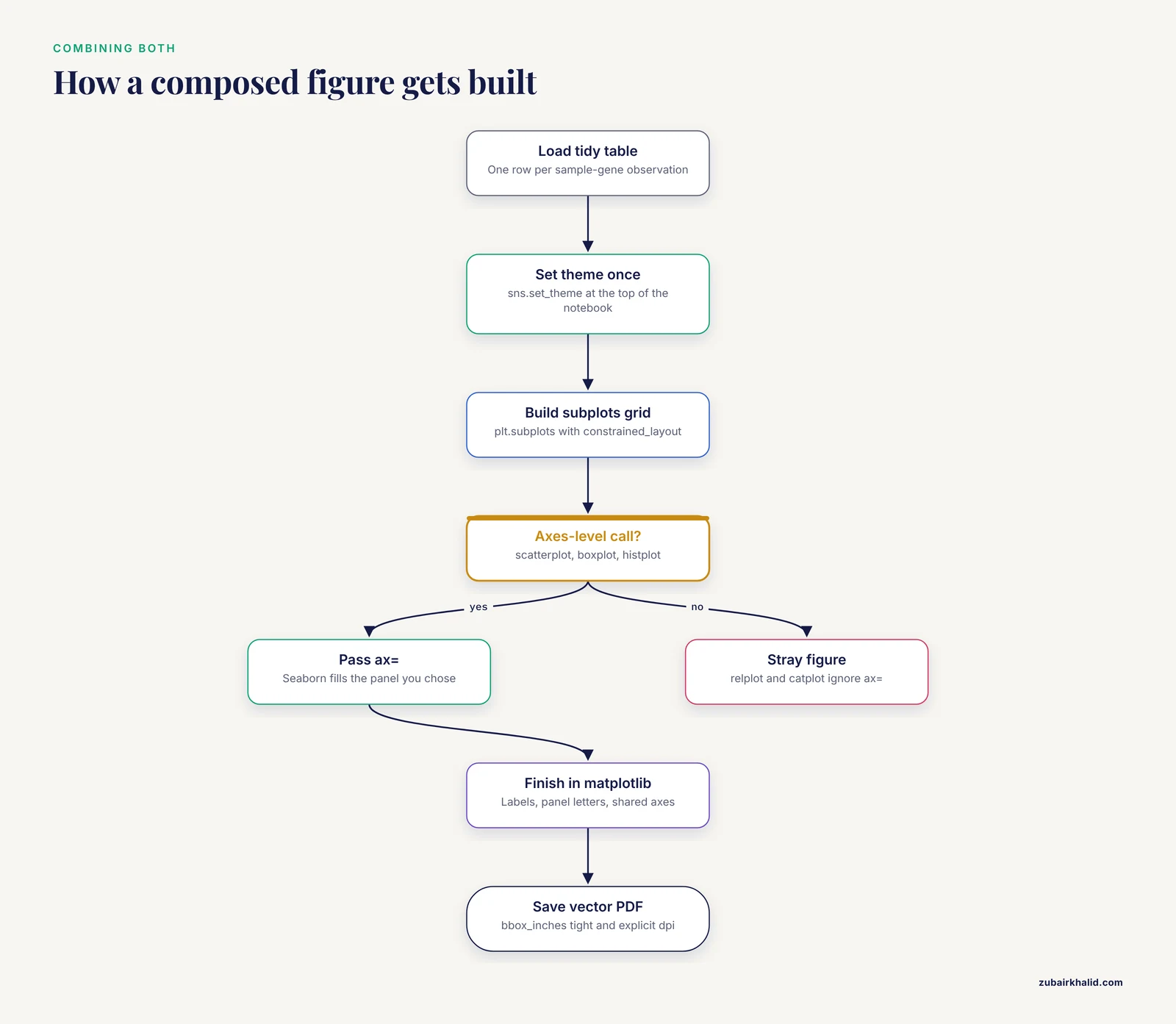
Because Seaborn returns matplotlib objects, the two compose cleanly. The pattern below shows a realistic QC-plus-figure block for a small expression experiment.
import matplotlib.pyplot as plt
import seaborn as sns
import pandas as pd

# Load a tidy table: one row per sample-gene observation
df = pd.read_csv("expression_long.csv")

# Apply Seaborn theming once, at the top of the notebook
sns.set_theme(style="whitegrid", palette="colorblind", font_scale=1.1)

# Exploratory pass: Seaborn
sns.boxplot(data=df, x="condition", y="log2_tpm", hue="batch")
sns.despine()

# Publication pass: matplotlib composes panels, Seaborn fills them
fig, axes = plt.subplots(1, 2, figsize=(8, 3.5), constrained_layout=True)

sns.boxplot(data=df, x="condition", y="log2_tpm", ax=axes)
axes.set_ylabel("log2 TPM")
axes.set_xlabel("")

axes[1].scatter(df["gc_content"], df["log2_tpm"], s=12, alpha=0.6)
axes[1].set_xlabel("GC content")
axes[1].set_ylabel("")

fig.suptitle("Expression QC and sequence dependence")
fig.savefig("figure_1.pdf", dpi=300, bbox_inches="tight")
Three habits make this pattern reliable:
- Call
sns.set_theme()once at the top so every figure in the session shares style. - Pass
ax=to every Seaborn call inside a composed figure, because figure-level Seaborn functions create their own Figure and will not merge into yours. - Save with
bbox_inches="tight"and explicitdpi, and prefer PDF or SVG for vector output in submissions.
Setting Up a Reproducible Plotting Environment
A minimal, standard setup for a bioinformatics project:
# with pip
pip install matplotlib seaborn pandas numpy jupyterlab

# with conda, which is common in bioinformatics
conda install -c conda-forge matplotlib seaborn pandas numpy jupyterlab
Then in your first notebook cell:
import matplotlib.pyplot as plt
import seaborn as sns

sns.set_theme(context="paper", style="ticks", palette="colorblind")
plt.rcParams["svg.fonttype"] = "none"  # keep text as text in SVG for journals
Jupyter notebooks are the standard substrate for this work in biology. The protein data workshop described earlier is built entirely as a notebook-based activity, with starter and completed versions released so learners can check their own work [1], and that structure is worth copying for any internal lab tutorial you write.
Common Mistakes and Limitations
These are the errors that cost real time or, worse, produce misleading figures.
- Treating Seaborn and matplotlib as alternatives. Seaborn calls matplotlib to draw. Debugging a Seaborn plot ultimately means reading matplotlib state. New analysts who refuse to learn matplotlib hit a hard wall the first time a legend lands in the wrong place or a colorbar disappears.
- Mixing figure-level and axes-level Seaborn functions. Figure-level functions such as
relplot,catplot,displot, andjointplotcreate their own Figure and ignore anax=argument. Calling them inside aplt.subplots()grid silently produces a stray extra figure. Use the axes-level equivalents (scatterplot,boxplot,histplot) inside composed figures. - Reading too much into 2D embedding scatter plots. Visual inspection of two-dimensional representations such as PCA or UMAP plots for batch effects or condition separation is unstable and prone to confirmation bias. The scXMatch project was created precisely to replace that visual habit with a principled non-parametric graph-based test for distribution shifts in single-cell data, validated on gene expression, chromatin accessibility, and imaging-derived morphology [17]. Plot the embedding for communication, but test the shift statistically.
- Letting categorical order drift. Seaborn plots categories in the order it meets them unless you pass an explicit
order=argument. Two panels built from differently filtered DataFrames can show the same conditions in different colors and orders, which misleads readers badly. Fix orders and palettes with dictionaries keyed on category names. - Overplotting dense biological data. Single-cell datasets, per-base genome tracks, and high-throughput screens produce point clouds where default scatter rendering hides the actual density. Use 2D histograms, hexbin, kernel density plots, or
rasterized=Truefor large scatter layers in vector output. - Ignoring color accessibility and journal norms. Default rainbow-style colormaps distort perception of continuous data. Use perceptually uniform colormaps (viridis and its relatives) for continuous quantities and Seaborn's colorblind palettes for categorical ones, and check figures in grayscale before submission.
- Assuming defaults are stable across versions. Matplotlib and Seaborn both evolve their default styles and API. A figure regenerated two years later with unpinned versions can look different. Pin library versions in
requirements.txtor an environment file for every analysis that produces a manuscript figure. - Forgetting that statistics must live upstream. Neither library decides whether a difference is significant. Compute tests in your analysis code, then draw the result. A p-value drawn on a plot as an annotation is only as honest as the test behind it, and that test is your responsibility, not the plotting library's.
A final scope note: this article covers the plotting layer only. Tool choice for upstream steps, from alignment through statistical modeling, follows the same principle of matching the tool to the data shape, but those choices are separate decisions documented in the respective tool literature.
Frequently Asked Questions
Should I learn matplotlib or seaborn first for bioinformatics?
Learn Seaborn first if your immediate work is exploring tables of biological data, then learn matplotlib as soon as you need to customize anything. Seaborn's faster feedback keeps beginners moving, but every Seaborn plot is a matplotlib object, so matplotlib knowledge is unavoidable for publication work and is what makes custom scientific graphics possible at all.
Can I use matplotlib and seaborn together in the same figure?
Yes, and you should. Seaborn is built on matplotlib, so calling sns.boxplot(ax=axes) fills one panel of a matplotlib figure while axes[1].imshow() fills another with an image. The one rule is to use axes-level Seaborn functions, not figure-level functions such as catplot, when composing multi-panel figures.
Which library produces publication-quality figures?
Both can, because Seaborn output is fully editable through matplotlib after drawing. Matplotlib gives you the control needed for exact journal specifications, fonts, panel labels, and multipanel layouts, while Seaborn gets individual panels close to final quality faster. In practice, figures are composed in matplotlib with Seaborn supplying the statistical panels.
Does seaborn work with the DataFrames my bioinformatics pipeline produces?
Yes. Seaborn is designed around tidy pandas DataFrames, which is what BioPythony parsers, scikit-learn pipelines, and most omics tools output once you assemble results into long-format tables. If your results are nested dicts or matrices, reshape them with pandas into one-row-per-observation format and Seaborn's column-name-based API applies directly.
Is matplotlib enough for single-cell RNA-seq data?
Matplotlib plus Seaborn covers the standard single-cell QC and summary plots, including quality metric distributions, embedding scatters, and marker heatmaps. Dense embeddings need careful handling of overplotting, and formal claims about distribution shifts between conditions should rest on statistical tests rather than visual inspection of embeddings alone.
Do I need to understand matplotlib internals to fix ugly seaborn plots?
You need the basics, not the internals. Knowing that a Seaborn function returns a matplotlib Axes, and that Axes methods such as set_xlabel, set_ylim, tick_params, and legend adjust the result, resolves the large majority of styling complaints. Deep internals (transforms, custom artists, projection classes) only matter for highly custom graphics.
Sources
- Visualizing protein big data using Python and Jupyter notebooks.
- Large-Scale Data Analysis of Post-Traumatic Stress Disorder (PTSD) Through GWAS Fine-Mapping and Systems Biology.
- Blender tissue cartography: an intuitive tool for analyzing 3D microscopy data.
- ScaleBarOn and Muad'Data: simple Python tools for elemental imaging data visualization and comparative scaling.
- QuickProcess2: an integrated package for crystallography data visualization, processing and management at the GM/CA Structural Biology Facility.
- PySimi: a unified framework for similarity measure evaluation in spectral clustering with applications to omics data.
- sortscore: Sort-seq MAVE scoring and visualization using Python.
- A Protocol for Multivariate Data Visualization and Pseudotime Modeling for Analysis of Disease Trajectories Detected by Mass Spectrometry Imaging.
- seqme: a Python library for evaluating biological sequence design from generative models.
- PhenoFECT: A Python package for forecasting and exploring plant phenology under climate change.
- PerSeqPIPE: Nextflow workflow for per-sequence analysis of small RNA-sequencing data.
- FetchPA: a guided, end-to-end solution for local ATAC-Seq data processing and analyses.
- An Integrated Ecosystem for Analysis and Visualization of Large-Scale Phylogenomic Data Combining ETE Toolkit, TreeProfiler, and PhyloCloud for Scalable Phylogenomic Analysis.
- PhyloZoo: a unified framework for phylogenetic network analysis in Python.
- Fast-nnt: fast, reproducible, and scalable neighbour network analysis in R, Python, and CLI.
- Computational Tools for LC-IMS-MS Data Processing in Metabolomics.
- Quantifying distribution shifts in single-cell data with scXMatch.