How to Set Up Jupyter Notebook for Bioinformatics

By Dr. Zubair Khalid, DVM, MS, PhD · 2026-11-11

By the end of this jupyter notebook bioinformatics tutorial you will have a working, isolated Python environment on your own machine, JupyterLab running in your browser, and a notebook that downloads a real nucleotide record from NCBI, parses it with Biopython, calculates GC content, and plots base composition. You will also know how to register a custom kernel, freeze your environment for reproducibility, and avoid the errors that trip up most people during their first week of setting up Jupyter for bioinformatics.

Here is what you need before you start:

• A laptop or desktop running macOS, Linux, or Windows. Any machine from roughly the last six years is fine. About 8 GB of RAM keeps you comfortable for notebooks, plotting, and moderate data work.
• Roughly 5 GB of free disk space for Miniconda and one environment with common bioinformatics packages.
• A terminal. On macOS and Linux this is Terminal or any shell. On Windows, use PowerShell or, better, the Git Bash terminal that ships with Git for Windows.
• An internet connection, because you will download an installer and packages from package repositories.
• No prior Python experience is required for the setup itself, although the worked examples assume you can read basic Python.

Why Jupyter Notebook Fits Bioinformatics Work

A Jupyter notebook is a browser-based document that mixes executable code, its output, narrative text, and figures in a single file. That structure matches how bioinformatics work actually happens. You run a chunk of analysis, look at a table or a plot, adjust the parameters, and run again. The final document doubles as a lab notebook and a methods section.

The published literature backs this pattern across subfields. Interactive Jupyter notebooks have been used to teach protein dynamics network analysis from molecular dynamics simulations, with the workflow designed to scale from small prototype proteins to large membrane proteins [1]. In metabolomics, researchers have promoted notebook-based interactive computational lab notebooks as a way to make omics analyses transparent, reusable, and aligned with FAIR data principles [2]. Reproducibility case studies in bioinformatics have converged on the same recommendation, offering a Jupyter notebook walkthrough as one of the primary ways to re-execute and verify a published analysis [3]. Entire pipelines, including an open RNA-seq workflow with alignment, PCA, clustering, and enrichment analysis, have been distributed as notebooks paired with Docker images so that non-experts can run them with minimal configuration [4]. Specialized packages such as ssbio even render protein structures and genome-scale model annotations directly inside notebook cells [5].

None of that works, though, if the environment underneath the notebook is a mess. The single biggest cause of broken bioinformatics notebooks is a Python installation that mixes system packages, pip installs, and conda packages until nothing resolves. The setup below avoids that from the first command.

What You Need to Know Before Running Commands

Two vocabulary items come up constantly:

• Environment. A self-contained directory holding a specific Python interpreter and a specific set of packages. Environments let you keep a project pinned to Biopython 1.83 while another project uses something newer, without the installs interfering.
• Kernel. The running process that actually executes the code in your notebook cells. One environment can power one kernel, and each notebook session attaches to exactly one kernel. Most "my package is missing" errors are really "my notebook is attached to the wrong kernel" errors.

We will use Miniconda, a minimal installer for the conda package manager. Conda handles both Python packages and compiled command-line bioinformatics tools, and it resolves binary dependencies so tools like Biopython and matplotlib install with their C extensions intact. Alternative managers such as mamba (a faster conda-compatible drop-in) and pip (Python-only) appear later in this guide where they fit.

Step-by-Step Setup

Step 1: Install Miniconda

Download and run the Miniconda installer for your operating system.

On macOS (Apple Silicon), run:

curl -O https://repo.anaconda.com/miniconda/Miniconda3-latest-MacOSX-arm64.sh
bash Miniconda3-latest-MacOSX-arm64.sh

On Linux:

wget https://repo.anaconda.com/miniconda/Miniconda3-latest-Linux-x86_64.sh
bash Miniconda3-latest-Linux-x86_64.sh

On Windows, download the latest Miniconda3 Windows 64-bit installer from the Miniconda documentation page and run it, accepting the defaults. Check the box to add Miniconda to your PATH environment variable only if you know what that means. If you leave it unchecked, launch conda from the "Anaconda Prompt" shortcut that the installer creates.

During the macOS and Linux install, accept the license, accept the default install location, and answer yes when asked whether to run conda init. Then close and reopen your terminal and verify:

conda --version

Expected output looks like this, where the exact build number will differ:

conda 24.7.1

If you see command not found: conda, the shell has not picked up the new initialization. Reopen the terminal first. If it still fails, run the installer again and confirm you answered yes to conda init.

Step 2: Create a Dedicated Bioinformatics Environment

Never install bioinformatics packages into the base environment. Create one environment per project. For this tutorial, create an environment named bioinfo with a current Python:

conda create -n bioinfo python=3.12

Parameters that matter:

• -n bioinfo sets the environment name. Choose names you will recognize six months from now, such as rnaseq-2026 or genome-annotation.
• python=3.12 pins the Python minor version. Pinning is deliberate. Some compiled bioinformatics wheels lag behind the newest Python, and a pinned version makes your environment.yml file reproducible later.

Conda will print a list of packages to install and ask for confirmation. Type y and press Enter. Expected output ends with lines like:

Proceed with package installation? [y/N] y
Preparing transaction: done
Executing transaction: done
#
# To activate this environment, use
#     $ conda activate bioinfo
#

Activate it:

conda activate bioinfo

When activation succeeds, your shell prompt gains a prefix:

(bioinfo) yourname@yourmachine ~ %

That prefix is your constant signal that the terminal is pointed at the right environment. Every pip or conda install from this point happens inside bioinfo and touches nothing else on your system.

Step 3: Install Jupyter and Core Bioinformatics Packages

Install everything from the conda-forge channel, which is the community standard for reproducible conda builds:

conda install -c conda-forge jupyterlab biopython pandas numpy matplotlib seaborn scipy

What each package does:

• jupyterlab installs the JupyterLab interface, the modern successor to the classic Notebook interface. Both jupyter lab and jupyter notebook commands remain available after this install.
• biopython is the foundational Python library for biological data. It parses FASTA, FASTQ, GenBank, and PDB files, talks to NCBI databases over the internet, wraps pairwise alignment, and handles sequence objects. Most python for bioinformatics work starts here.
• pandas holds tabular data such as count matrices and annotation tables.
• numpy and scipy provide numerical and statistical primitives.
• matplotlib and seaborn produce the figures you will embed in notebooks.

The install takes a few minutes. Conda prints a solving report, then an installation list. When it finishes, verify Biopython from the shell:

python -c "import Bio; print(Bio.__version__)"

Expected output:

1.84

The exact version number will differ as Biopython releases updates. Any version number means the import worked. A traceback here means the install did not land in the environment you think you are in, so re-run conda activate bioinfo and try again.

If a package you want is not on conda-forge, install it with pip from inside the activated environment:

pip install somepackage

Step 4: Register the Environment as a Jupyter Kernel

This step is the one most jupyter notebook bioinformatics tutorials skip, and it is the source of the most common error message in the whole ecosystem. Install the ipykernel package, then register the environment under a human-readable name:

conda install -c conda-forge ipykernel
python -m ipykernel install --user --name bioinfo --display-name "Python (bioinfo)"

Parameters that matter:

• -user installs the kernel specification in your home directory, so you do not need administrator rights.
• -name bioinfo is the internal identifier Jupyter uses. Keep it lowercase with no spaces.
• -display-name "Python (bioinfo)" is the name you will see in the Jupyter interface. The parentheses convention marks it as a conda environment rather than the system Python.

Expected output:

Installed kernelspec bioinfo in /Users/yourname/Library/Jupyter/kernels/bioinfo

The path varies by operating system. On Linux it typically lives under ~/.local/share/jupyter/kernels/, and on Windows under %APPDATA%\jupyter\kernels\.

Why this matters: if you launch Jupyter from within an activated environment, the default python3 kernel often points at that environment anyway. But if you later launch Jupyter from base or from another project, only a registered kernel guarantees that a notebook opened next month still finds your packages. Registering the kernel decouples the notebook from however you happened to launch Jupyter that day.

Step 5: Launch JupyterLab and Verify the Setup

From your terminal, still in the bioinfo environment:

jupyter lab

Your default browser opens at an address like http://localhost:8888/lab, and the terminal shows a startup log including a tokenized URL. The token lets you reconnect if the browser tab is lost. Copy the URL from the terminal if the browser does not open automatically.

In JupyterLab, create a new notebook: File, New, Notebook. When prompted to select a kernel, choose Python (bioinfo), the display name you registered in Step 4.

Now run the verification cell. Paste this into the first cell and press Shift+Enter:

import sys
print(sys.executable)
import Bio
import pandas
import matplotlib
print("Biopython", Bio.__version__)
print("pandas", pandas.__version__)
print("matplotlib", matplotlib.__version__)

Expected output:

/Users/yourname/miniconda3/envs/bioinfo/bin/python
Biopython 1.84
pandas 2.2.2
matplotlib 3.9.1

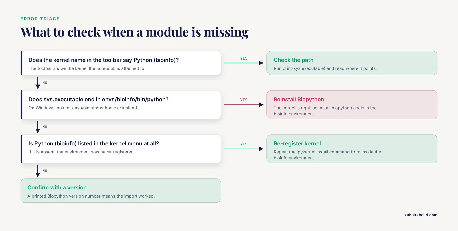
Check the first line carefully. It must end in envs/bioinfo/bin/python (or envs\bioinfo\python.exe on Windows). If it points somewhere else, the notebook is attached to the wrong kernel. Click the kernel name in the top-right corner of JupyterLab, switch to Python (bioinfo), and re-run.

Step 6: First Biopython Exercise, Downloading From NCBI

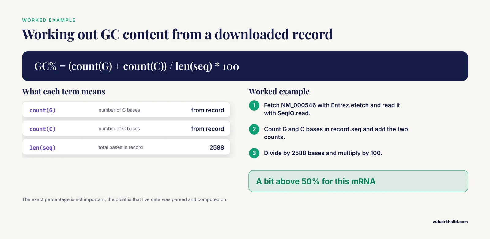
With the environment verified, run a real analysis. The following biopython tutorial-style cells fetch a reference mRNA sequence from the NCBI Nucleotide database over the internet, so they require connectivity.

NCBI asks programmatic users to identify themselves with an email address. Set it before any network call:

from Bio import Entrez, SeqIO
Entrez.email = "[email protected]"

Fetch the reference mRNA record for the human TP53 gene (accession NM_000546):

handle = Entrez.efetch(
    db="nucleotide",
    id="NM_000546",
    rettype="fasta",
    retmode="text",
)
record = SeqIO.read(handle, "fasta")
handle.close()

print(record.id)
print(record.description)
print(len(record.seq), "bases")

Expected output resembles:

NM_000546.6
Homo sapiens [transcription factor](/knowledge/molecular-biology/transcription-factor) p53 (TP53), transcript variant 1, mRNA
2588 bases

The version suffix on the accession and the exact length depend on which record revision NCBI serves. What matters is that you get an accession, a species and gene description, and a length in the low thousands of bases for this transcript.

Now calculate GC content. The formula is the count of G and C bases divided by total length, times 100:

seq = record.seq
gc_percent = (seq.count("G") + seq.count("C")) / len(seq) * 100
print(f"GC content: {gc_percent:.1f}%")

For a mammalian mRNA like this one, expect a GC percentage a bit above 50. The precise number is not important. What matters is that you just downloaded live data from a public database, parsed it into a Biopython sequence object, and computed on it in under ten lines, all inside a document that recorded every step.

Step 7: Parse a Local FASTA File and Plot Base Composition

Most bioinformatics work happens on local files, so practice the pattern you will use every day. Create a file called reads.fasta in the same folder as your notebook, with this content:

>read1 synthetic_sequence_for_tutorial
ATGCGATCGATCGGGCTA
>read2 synthetic_sequence_for_tutorial
GGCCTTAAGGCATTACG
>read3 synthetic_sequence_for_tutorial
TTAACGCGGATCCGTAAT

This toy FASTA uses short synthetic sequences so you can eyeball the answer. Parse and summarize it:

from Bio.SeqUtils import gc_fraction

for record in SeqIO.parse("reads.fasta", "fasta"):
    print(record.id, len(record.seq), f"GC {gc_fraction(record.seq) * 100:.1f}%")

Expected output:

read1 18 GC 55.6%
read2 18 GC 50.0%
read3 18 GC 44.4%

Note the modern function name. gc_fraction was introduced in recent Biopython releases and returns a fraction between 0 and 1, which is why the example multiplies by 100. Older code you find online uses Bio.SeqUtils.gc_content, and if you copy such code into a current install you will get an import error. This version drift is normal in active libraries and is one more reason to pin versions per project.

Now plot base composition across the three reads with matplotlib:

import matplotlib.pyplot as plt

ids, counts_a, counts_t, counts_g, counts_c = [], [], [], [], []

for record in SeqIO.parse("reads.fasta", "fasta"):
    s = record.seq
    ids.append(record.id)
    counts_a.append(s.count("A"))
    counts_t.append(s.count("T"))
    counts_g.append(s.count("G"))
    counts_c.append(s.count("C"))

fig, ax = plt.subplots()
bottom =  * len(ids)
for counts, base, label in [
    (counts_a, "A", "A"),
    (counts_t, "T", "T"),
    (counts_g, "G", "G"),
    (counts_c, "C", "C"),
]:
    ax.bar(ids, counts, bottom=bottom, label=label)
    bottom = [b + c for b, c in zip(bottom, counts)]

ax.set_ylabel("Base count")
ax.set_xlabel("Read")
ax.legend(title="Base")
plt.show()

You should see a stacked bar chart with one bar per read, colored by base, and every read totaling 18. The figure is embedded in the notebook, so the notebook now contains the question, the code, and the answer in one artifact.

Step 8: Freeze and Share the Environment

The final step of setting up Jupyter notebook for bioinformatics properly is making the setup survive. From the activated environment, export it:

conda env export > environment.yml

Keep environment.yml next to your notebooks, ideally in a Git repository. Anyone (including you, on a new machine or after a disk failure) can rebuild the exact environment:

conda env create -f environment.yml
conda activate bioinfo

For sharing a single notebook with an interactive session rather than a file, Binder builds a live environment from your repository on demand. The ssbio project distributes its structural biology notebooks this way, letting readers launch and run the tutorial code in a browser without installing anything [5].

Command and Option Reference

Jupyter Notebook Bioinformatics Tutorial Tips

These are the habits that separate a notebook you can build on from a notebook that breaks in a month.

Restart and run all before you share. The Kernel menu in JupyterLab has "Restart Kernel and Run All Cells". Executed top to bottom, your notebook must produce its own results. Notebooks allow out-of-order execution, which means a file that looks fine can depend on a cell you deleted an hour ago. Running the full document catches that before a collaborator does.

Install packages in the terminal, not in notebook cells. Copying pip install lines into cells feels convenient and quietly breaks reproducibility, because the environment the notebook describes no longer matches any environment.yml. If you must install from a cell, use the %pip install line magic, which guarantees the install targets the notebook's own kernel.

Keep paths relative and data outside the repository. Reference data/sample.fastq relative to the notebook, never /Users/yourname/old-project/data/sample.fastq. Absolute paths are the top reason a notebook runs on your machine and nowhere else. Add raw data directories to .gitignore and document where to download inputs.

Use notebooks for orchestration and visualization, scripts for heavy lifting. Notebooks are excellent for exploratory data analysis, plotting, parameter tuning, and gluing tools together. Cell-by-cell interactive execution becomes a liability for jobs that run for hours or process millions of reads. Published pipeline examples handle this by treating the notebook as the driver and the heavy alignment steps as platform-independent components, sometimes packaged with Docker so compute can move to suitable hardware [4]. If an analysis will scale up, write the core loop as a script that the notebook calls.

Pin versions and record the environment in the narrative. A markdown cell at the top of the notebook stating the key package versions, the date, and the input file versions costs nothing and saves hours. The reproducibility literature shows that even with code and data available, missing details about versions and configuration can make a published method hard to re-run, which is exactly the failure mode this habit prevents [3].

Use nbdime for version control diffs. Plain Git diffs of .ipynb files are unreadable because they embed JSON output blobs. The nbdime tool (installable with pip or conda) diffs and merges notebooks cell by cell, showing code changes and ignoring output churn. It also provides git nbdiff and git nbmerge integration.

Learn the cell magics that matter for bioinformatics. %timeit code times a single line across repeated runs. %%bash runs an entire cell as a shell script, which is handy for calling samtools, bwa, or other command-line tools installed in the same conda environment. %%capture suppresses verbose tool output you do not want saved in the notebook file.

Structure notebooks like a methods section. Lead with a markdown cell stating the goal, inputs, and outputs. Use headers to separate fetching, QC, analysis, and figures. The metabolomics community's push toward notebook-based computational lab notebooks is at heart a documentation argument, since a well-structured notebook is readable by reviewers and colleagues without running anything [2].

Set your Entrez email and respect NCBI limits. Biopython's network calls to NCBI are rate-limited by the service. Identify yourself with Entrez.email, batch requests where possible, and do not loop thousands of fetches in a tight cell. For bulk retrieval, NCBI's FTP and mirror resources are the right tools.

Troubleshooting: Exact Errors and Fixes

ModuleNotFoundError: No module named 'Bio'

The most common error in python for bioinformatics. The notebook's kernel is not the environment where Biopython is installed. Fix: check the kernel name in the JupyterLab toolbar, switch to Python (bioinfo), and re-run. If the kernel is not listed at all, repeat Step 4. Confirm with print(sys.executable) that the path ends in your environment directory.

zsh: command not found: conda (or bash: conda: command not found)

Conda is not initialized in the current shell. Reopen the terminal. If it persists, re-run the Miniconda installer or run source ~/miniconda3/bin/activate followed by conda init for your shell, then reopen the terminal.

jupyter: command not found

JupyterLab is installed in the bioinfo environment but you launched the terminal command from base or another environment. Run conda activate bioinfo first. Alternatively, launch from anywhere if you installed Jupyter globally, then select the bioinfo kernel inside the interface.

Port 8888 is already in use

Another Jupyter server is already running, often from a forgotten terminal window. Either use that existing server (check your browser tabs and terminal history) or start a new one on another port with jupyter lab, port=8889.

ImportError: cannot import name 'Seq' from 'Bio' (most likely due to a circular import)

You named one of your own files Bio.py or bio.py in the working directory, and Python is importing your file instead of the library. Rename your file and delete the accompanying pycache folder.

EnvironmentLocationNotFound: Not a conda environment when switching kernels

The kernel spec registered in Step 4 points at an environment that was deleted or renamed. Re-register the kernel from inside the existing environment.

Conda solver runs for many minutes or reports UnsatisfiableError

You are likely mixing channels or mixing conda and pip for the same packages. Cancel, then create a fresh environment and install from conda-forge first. Add pip-only packages afterward, and never re-install a conda package with pip in the same environment.

Plots do not appear in older classic notebooks

In the classic Notebook interface, add %matplotlib inline as the first line of the plotting cell. JupyterLab renders figures automatically without the magic.

Common Mistakes and Limitations

Beyond one-off errors, these are the systemic mistakes people make when setting up Jupyter notebook for bioinformatics.

Working in base. Every package you install in base raises the odds of a future solver conflict that breaks all projects at once. It costs one command to make an environment. Make one.

Not registering kernels. As covered in Step 4, skipping kernel registration ties notebook behavior to launch context, which produces notebooks that "work on my machine" and fail everywhere else.

Committing outputs and large data. A notebook with embedded PNG figures and a saved table can balloon to tens of megabytes, which chokes Git. Clear outputs before committing, or configure a tool like nbstripout to do it automatically, and keep raw data files out of the repository.

Trusting a notebook that was never run end to end. Out-of-order execution means the visible state of a notebook can hide dependencies on deleted variables. "Restart and Run All" is the only trustworthy state.

Assuming notebooks scale to everything. Jupyter is a superb interactive layer over bioinformatics tooling. It is not a workflow manager. Analyses spanning many samples, many steps, and reruns on updated data belong in a pipeline framework, with the notebook serving as the interface for inspection and figure generation. The RNA-seq pipeline literature shows the notebook-plus-container pattern working well precisely because the heavy steps are encapsulated and movable to adequate hardware [4].

Ignoring the reporting layer. A notebook only improves reproducibility if the surrounding project is disciplined about versions, inputs, and documentation. The reproducibility case study literature is blunt that code availability alone does not guarantee re-execution, and recommends pairing code with a step-by-step runnable walkthrough and, where practical, containerization [3].

One limitation to name plainly. A tutorial environment cannot validate your biological interpretation. It gives you the tooling to run analyses correctly and document them, but design choices, statistical assumptions, and biological conclusions remain your responsibility, and unusual datasets deserve review by someone with domain expertise before results feed into a manuscript or a clinical decision.

Frequently Asked Questions

Jupyter Notebook and JupyterLab, which one should I install?

Install JupyterLab. It is the current standard interface, and it includes the classic Notebook as a compatible file format, so any .ipynb file opens in either. The jupyter notebook command still works and launches the older interface, which some older tutorials prefer, but everything in this guide runs in JupyterLab.

Do I need conda, or can I just use pip?

You can use pip with a virtual environment via the built-in venv module, and it works fine for pure-Python work. Conda earns its complexity in bioinformatics because many tools ship compiled dependencies and because conda-forge also distributes non-Python command-line tools such as samtools and bwa that notebooks commonly call. For a first setup, conda is the lower-friction path.

How do I install Biopython and confirm it works?

Inside your activated environment, run conda install -c conda-forge biopython, then verify with python -c "import Bio; print(Bio.version)". A version number confirms success. The worked example in Step 6 doubles as a functional test, since it exercises parsing and network access.

Why does my notebook say a module is missing even though I installed it?

Your notebook is attached to a different kernel than the environment where you installed the package. This happens when you install in the terminal but launch Jupyter from another environment. Fix it by registering the environment as a kernel and selecting that kernel in the notebook, as described in Steps 4 and 5.

Can I run Jupyter on an HPC cluster or a remote server?

Yes. The usual pattern is to run jupyter lab on the remote node, which prints a URL with a token, then create an SSH tunnel from your laptop to that port and open the tunneled URL in your local browser. Many clusters also provide Jupyter through a web portal such as Open OnDemand. Check your institution's documentation, since port forwarding rules vary by system.

How should I handle large files like FASTQ and BAM in a notebook?

Do not load them into memory. Stream them line by line or record by record (Biopython's SeqIO.parse is a generator, so it reads one record at a time), use samtools or pysam to slice only the regions you need, and keep the notebook focused on summary statistics and plots. If a step needs hours of compute, move it to a script or a workflow manager and have the notebook read its output.

What is the easiest way to share a runnable notebook with a colleague?

Commit the notebook, the environment.yml, and a small test dataset to a Git repository, clear the outputs, and verify it passes Restart and Run All. For a live session, add a Binder link so the repository builds an executable environment in the browser, which is how projects like ssbio publish their interactive tutorials [5]. For static reading, export to HTML with nbconvert.

Is a notebook a good place to build a full pipeline?

For exploration and for modest end-to-end analyses, yes, and published pipelines have shipped successfully as notebooks [4]. For anything you will rerun on new data or run across many samples, keep the heavy steps as separate scripts or a workflow system and let the notebook orchestrate and visualize. That split keeps the interactive benefits without making long jobs fragile.

Sources

1. Concepts, Practices, and Interactive Tutorial for Allosteric Network Analysis of Molecular Dynamics Simulations.
2. Toward collaborative open data science in metabolomics using Jupyter Notebooks and cloud computing.
3. Experimenting with reproducibility: a case study of robustness in bioinformatics.
4. An open RNA-Seq data analysis pipeline tutorial with an example of reprocessing data from a recent Zika virus study.
5. ssbio: a Python framework for structural systems biology.