How to Move from Toy Datasets to Real Biological Data
By Dr. Zubair Khalid, DVM, MS, PhD ·

Every bioinformatics course starts the same way. You load the iris dataset, run a clustering function, get a clean plot, and move on. Then you download your first real dataset and everything stops working. Genes are missing. Metadata is a spreadsheet with three different spellings of the same condition. The matrix has 32,738 rows and 2,700 columns and none of the tutorial code runs on it.
This guide shows you how to make that jump deliberately instead of painfully. By the end you will be able to choose a real dataset from a public repository, load it into a reproducible environment, run a standard quality control and analysis pipeline, verify that your results match the biology and the original publication, and avoid the mistakes that trip up almost everyone on their first real analysis.
Here is what you need on hand before you start:
- Python 3.9 or newer, with
pipandvenv(both ship with Python) - About 8 GB of RAM and a normal internet connection
- A terminal or the Anaconda Prompt on Windows
- Optional but useful: R 4.x with Bioconductor, if you plan to work with bulk RNA-seq tools
- A notebook environment such as JupyterLab, which you will install in Step 1
The walkthrough uses real, publicly released human single-cell RNA-seq data. The same reasoning transfers to microbiome amplicon data, proteomics, and imaging data.
What Actually Changes When the Data Gets Real
Toy datasets are small, complete, and tidy. The iris dataset has 150 rows, 4 numeric columns, no missing values, and three balanced classes. Real biological data breaks every one of those assumptions at once.
First, dimensionality inverts. A toy dataset has a handful of features and many samples. A single-cell RNA-seq matrix can have tens of thousands of genes and hundreds to millions of cells. Working with such high-dimensional data has its own statistical and computational challenges that simple multivariate tutorials do not prepare you for [1]. Distances become less meaningful, variance is dominated by technical noise, and the intuition you built on four-column data does not carry over.
Second, the data is noisy and incomplete. Dropout in single-cell measurements, ambiguous mapping reads, and missing measurement values are normal, not exceptions. Methods designed for real data explicitly account for this. For example, diffusion maps adapted for single-cell data include uncertainty and missing measurement values in the model, because pretending the matrix is complete gives wrong trajectories [1].
Third, formats are a mess. Upstream tools export one format, downstream tools want another, and connecting them often requires writing custom scripts or hours of manual conversion work. This is a documented, systematic problem in microbiome analysis pipelines, where the lack of universal data formats makes tool integration one of the main barriers for newcomers [2]. The same pattern repeats across sequencing-based fields.
Fourth, biology is messier than the toy. In differentiation studies you do not get clean, well-separated clusters. Cells follow continuous, branching trajectories with stochasticity along the path, so a clustering tutorial will happily carve a smooth continuum into meaningless islands [1]. Real data asks you to think about what structure should exist before you run an algorithm that will find some structure regardless.
Understanding these four shifts is the core of moving from toy datasets to real data in bioinformatics. Everything in the walkthrough below is built to handle them.
Why a Bioinformatics Course Alone Is Not Enough
A good bioinformatics course teaches you algorithms, data structures, and statistics. That is necessary and you should not skip it. But courses concentrate the learning on clean inputs because that is where the concepts are clearest. The gap shows up in three places.
Method documentation assumes a technical audience. The details behind network-based tools and many other method families are often written for readers who already know the underlying graph theory and the implementation conventions. Interactive tutorial resources such as Graphery exist precisely to close this gap, pairing each graph concept with executable Python code that runs on real-world biological networks, without even requiring an account [3]. Seek out resources of that style when a method paper reads like math homework.
The command line is a wall for novices. Many end-to-end analysis platforms for sequencing data run entirely through a command line interface, and the steep learning curve is a real barrier for new researchers. This is why teaching curricula for real data, such as the PUMAA microbiome curriculum, deliberately design around the CLI bottleneck and focus classroom time on data analysis, visualization, and statistical reasoning rather than shell syntax [2]. You will eventually need the command line, but it should not be the first thing that blocks you.
Real analysis is mostly data wrangling. In a course, 90 percent of the work is done for you. With real data, loading the files correctly, aligning sample names, and verifying the metadata account for most of the hours. Planning for that reality, rather than feeling like you are failing at "the science," is half the battle.
The practical conclusion for anyone who wants to learn bioinformatics properly: treat courses as the map, then spend most of your deliberate practice driving on real roads.
Picking Your First Real Dataset
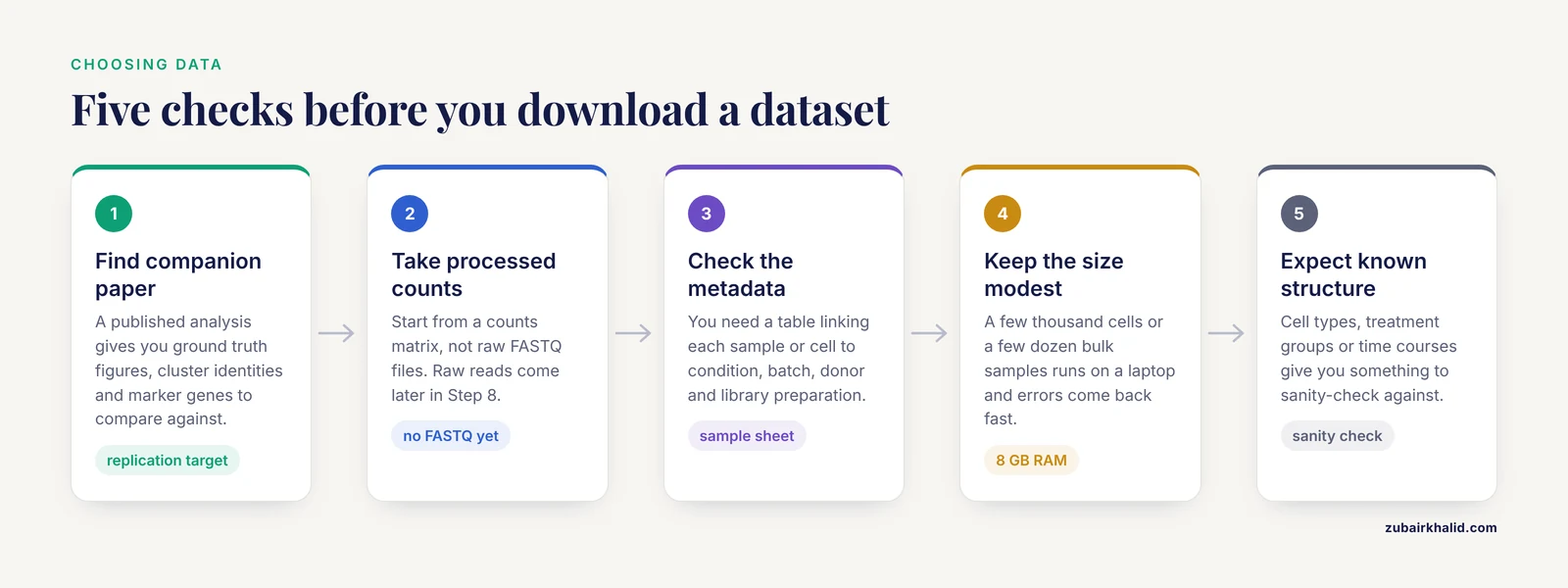
Not all real datasets are equally good first targets. Use these criteria when you choose.
- Published companion paper. If a paper analyzed the dataset, you have ground truth figures, cluster identities, and marker genes to compare against. This turns your analysis into a replication exercise with a known answer.
- Processed data available. Start with a dataset that ships a counts matrix, not raw FASTQ files. You can move to raw reads later. Gene counts matrices are standard outputs of upstream pipelines and are far easier to inspect.
- Good metadata. You need a table linking each sample or cell to its condition, batch, donor, and library preparation. Datasets with a sample sheet are worth twice the effort of datasets without one.
- Modest size. A few thousand cells or a few dozen bulk samples is ideal. It runs on a laptop and errors come back fast.
- A known biological structure. Cell types, treatment groups, or time courses give you something to sanity-check against.
Two datasets meet all five criteria and are used across the field precisely because they are real data in convenient packaging:
- pbmc3k: 2,700 human peripheral blood mononuclear cells from a 10x Genomics run. Real donor, real cells, real technical noise, bundled for programmatic download.
- airway: an eight-sample bulk RNA-seq experiment on human airway smooth muscle cells treated with dexamethasone, distributed through Bioconductor with its full metadata.
These are not simulations. They carry the exact problems you will face in your own data, which is why they work as a bridge.
Moving from Toy Datasets to Real Data, Step by Step
This is the core walkthrough. Work through it once with the commands exactly as written, then repeat it with a dataset you chose yourself.
Step 1: Set Up a Reproducible Environment
Never install analysis packages into your system Python. Create an isolated environment so that a package upgrade six months from now cannot silently break your analysis.
python -m venv bioenv
source bioenv/bin/activate      # Windows: bioenv\Scripts\activate
pip install scanpy leidenalg jupyterlab
You should see a series of lines starting with Successfully installed. Immediately record the versions:
pip freeze > requirements.txtThat one-line file is the beginning of reproducibility. Anyone, including future you, can rebuild the exact environment with pip install -r requirements.txt. Every step below assumes your prompt shows the activated (bioenv) prefix.
Step 2: Load a Real Dataset and Inspect Its Structure
Start JupyterLab with jupyter lab, open a notebook, and run:
import scanpy as sc

adata = sc.datasets.pbmc3k()
adata
Expected output:
AnnData object with n_obs × n_vars = 2700 × 32738
    var: 'gene_ids'
This object is an AnnData. Learn its anatomy, because every single-cell tool you will ever use speaks this format:
adata.Xholds the expression matrix. Here it is a sparse matrix of 2,700 cells by 32,738 genes, where most entries are zero. Sparse storage exists precisely because real data is mostly zeros.adata.obsis a table with one row per cell. QC metrics, cluster labels, and metadata land here.adata.varis a table with one row per gene. Gene symbols and flags such as mitochondrial status live here.adata.unsstores unstructured results like neighborhood graphs and markers.
Notice what already differs from a toy dataset: 32,738 features against 2,700 samples, and a matrix that cannot even be stored densely without wasting memory on zeros.
Step 3: Quality Control and Filtering
Real data always contains low-quality cells and uninformative genes. Filter both, but keep the filters conservative at first.
adata.var["mt"] = adata.var_names.str.startswith("MT-")
sc.pp.calculate_qc_metrics(adata, qc_vars=["mt"], percent_top=None, log1p=False, inplace=True)

sc.pp.filter_cells(adata, min_genes=200)
sc.pp.filter_genes(adata, min_cells=3)
Expected output for the gene filter:
filtered out 19024 genes that are detected in less than 3 cellsThat single message tells you something important about real data: over half of the gene rows in this matrix are noise-level detections. After the filter, roughly 13,700 genes remain.
Parameter by parameter:
min_genes=200drops cells with fewer than 200 detected genes. A cell that transcribed almost nothing is a lysis artifact or an empty droplet, not biology.min_cells=3drops genes detected in fewer than 3 cells. Genes seen in only one or two cells cannot support any statistical test.qc_vars=["mt"]computespct_counts_mt, the fraction of reads from mitochondrial genes. High values suggest a stressed or damaged cell.
Now inspect distributions instead of trusting thresholds blindly:
sc.pl.violin(adata, ["n_genes_by_counts", "total_counts", "pct_counts_mt"], multi_panel=True)A common, defensible starting point from the standard reference workflow is to keep cells with more than 200 and fewer than 2,500 detected genes and with mitochondrial fraction under 5 percent:
adata = adata[adata.obs.n_genes_by_counts < 2500, :]
adata = adata[adata.obs.pct_counts_mt < 5, :]
The correct thresholds vary by tissue and chemistry. The violin plots are how you justify whatever cutoff you choose.
Step 4: Normalize and Transform
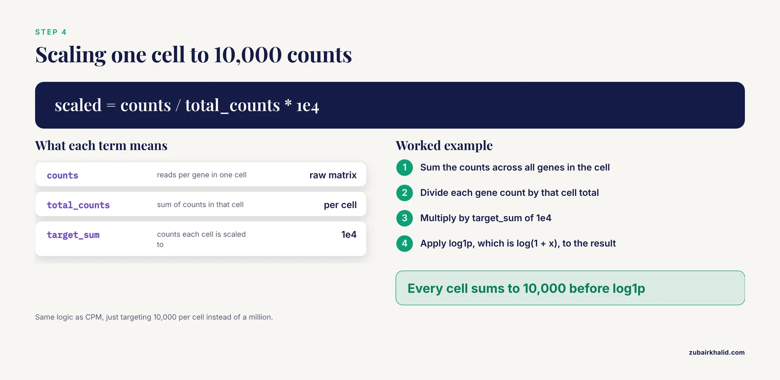
Two operations, each with a specific reason:
sc.pp.normalize_total(adata, target_sum=1e4)
sc.pp.log1p(adata)normalize_totalwithtarget_sum=1e4scales every cell so its counts sum to 10,000. This removes the effect of sequencing depth, so a cell that got twice as many reads does not look like it expressed twice as much. The formula is the same logic as CPM (counts per million), just targeting 10,000 per cell.log1papplies log(1 + x), compressing the long tail of expression values so that differences behave more like the assumptions of downstream statistics. The 1 offset avoids taking the log of zero, which happens constantly in sparse single-cell data.
Order matters. Normalizing before filtering wastes effort on genes you are about to delete, and log-transforming before depth normalization distorts the correction.
Step 5: Dimension Reduction
You cannot analyze 13,000 dimensions directly. Reduce them:
sc.pp.highly_variable_genes(adata, n_top_genes=2000)
sc.pp.scale(adata, max_value=10)
sc.tl.pca(adata, n_comps=50, svd_solver="arpack")
sc.pp.neighbors(adata, n_neighbors=10, n_pcs=30)
sc.tl.umap(adata)
sc.pl.umap(adata, color="pct_counts_mt")n_top_genes=2000keeps the most variable genes, which carry the biological signal. Keeping every gene would let low-information noise dilute the analysis.max_value=10clips extreme values after scaling so a single outlier gene cannot dominate the principal components.n_comps=50computes 50 principal components. You rarely need more, and checking the variance curve tells you how many carry real signal.n_neighbors=10andn_pcs=30define the neighborhood graph that UMAP and clustering both use. Lowern_neighborsproduces more local, fragmented structure. Higher values produce smoother global structure.
A note on method choice: PCA and UMAP are the default tools, but they are not the only option, and the right choice depends on the structure you expect. For differentiation data where cells move continuously through transcriptional state space rather than forming discrete groups, diffusion maps were developed specifically to produce a pseudotemporal ordering of single cells in high-dimensional gene expression space [1]. Choosing the dimension reduction method to match the biological question is a hallmark of working with real data rather than a toy.
Step 6: Cluster and Identify Marker Genes
sc.tl.leiden(adata, resolution=1.0, key_added="leiden", flavor="igraph", n_iterations=2)
sc.tl.rank_genes_groups(adata, "leiden", method="wilcoxon")
sc.get.rank_genes_groups_df(adata, group="0").head(10)
Expected output for the last line is a table with columns names, scores, pvals, pvals_adj, and logfoldchanges, listing the top genes that define cluster 0. On pbmc3k, cluster 0 is dominated by T-cell genes such as CD3D and CD3E.
resolution=1.0is the aggressiveness of clustering. Higher values produce more, smaller clusters. Adjust it against biology, not against prettier UMAP colors.method="wilcoxon"ranks genes per cluster by a rank-sum test. Simpler and more robust than most alternatives for a first analysis.
Annotate clusters by matching the top markers to known cell-type genes. On this dataset the expected picture is T cells (CD3D), B cells (MS4A1), monocytes (LYZ, FTL), natural killer cells (NKG7), and dendritic cells (CST3). If a cluster's top genes are ribosomal or mitochondrial rather than cell-type markers, suspect that cluster's quality rather than inventing a cell type for it.
Step 7: Sanity-Check Against the Original Publication
This step is what separates a real analysis from a tutorial copy. Open the publication that first described this data and compare three things:
- Cell-type composition. Do your cluster proportions roughly match the reported proportions of T cells, B cells, and monocytes?
- Marker genes. Do the same genes top your marker lists?
- Known biology. T cells should express
CD3D. B cells should expressMS4A1. If your "T cell" cluster is defined byLYZ, your cluster labels or your pipeline are wrong somewhere.
If all three line up, you have not just run code. You have reproduced a published result on real data, which is exactly the skill that matters.
Step 8: Graduate to Rawer Data
Once the processed-data pipeline feels routine, deliberately add friction. Download raw FASTQ files for a small experiment, run quality assessment on the reads, align or pseudoalign them, count transcripts per gene, and feed the resulting count matrix into the same downstream workflow you just learned. Each added layer (adapter trimming, alignment, counting) is where real projects lose their data quality, and each is worth one focused practice cycle. For microbiome work, end-to-end platforms handle import, denoising, taxonomy assignment, and diversity analysis in one pipeline, and teaching curricula have been designed around exactly this kind of complete workflow for undergraduates [2]. Whichever domain you pick, the principle is identical: incrementally move upstream until you can start from raw reads with confidence.
If you work in R, the same bridge exists for bulk RNA-seq:
install.packages("BiocManager")
BiocManager::install(c("airway", "DESeq2"))

library(airway)
data(airway)
colData(airway)$dex
You should see a factor with eight entries alternating between untrt (untreated) and trt (treated), from human airway smooth muscle cells exposed to dexamethasone. A standard differential expression pass uses a design that accounts for the donor cell line and the treatment:
library(DESeq2)
dds <- DESeqDataSet(airway, design = ~ cell + dex)
dds <- DESeq(dds)
res <- results(dds)
head(res)
The results table gives baseMean, log2FoldChange, lfcSE, stat, pvalue, and padj for every gene. The padj column, the adjusted p-value, is the one to filter on, because thousands of simultaneous tests guarantee many unadjusted false positives.
A Reference Table of Core Choices
Keep this table next to your keyboard. It summarizes the decisions you make in nearly every transcriptomic analysis of real data.
| Method or parameter | What it does | Typical setting | Watch out for |
|---|---|---|---|
Total-count normalization, target_sum=1e4 | Scales each cell to 10,000 counts, removing depth differences | Nearly always for count data | Must precede log transform |
log1p(x) = log(1 + x) | Compresses expression range, handles zeros | After normalization | Never log raw counts before depth scaling |
| Median-of-ratios (DESeq2 style) | Size-factor estimation for bulk differential expression | Default in DESeq2 | Needs most genes to be mostly unchanged |
Highly variable genes, n_top_genes=2000 | Restricts analysis to informative genes | 1,000 to 3,000 for single cells | Selection must be inside the correct data layer |
PCA, n_comps=50 | Linear dimension reduction, denoising | 30 to 50 PCs for the graph | PCA coordinates are linear and can miss curved structure |
UMAP, n_neighbors=10 | Nonlinear visualization | 10 to 30 neighbors | Distances and cluster sizes are not quantitative |
| Diffusion maps | Pseudotemporal ordering for continuous trajectories [1] | Differentiation and continuum data | Wrong tool for cleanly separated populations |
| Wilcoxon rank-sum test | Marker gene ranking per cluster | Default for cluster markers | Needs normalized, logged data as input |
Adjusted p-value (padj) | Multiple-testing correction | Filter at your stated threshold | Never interpret raw p-values at genomic scale |
Checking That Your Result Is Right
Real data gives you no answer key, so you build your own verification habits.
Replicate something published. As in Step 7, matching a published figure, a known marker set, or a reported proportion is the strongest cheap check available.
Use QC metrics as a scoreboard. After filtering, the mitochondrial percentage distribution should shift down, and the top principal component should no longer be dominated by total counts per cell.
Test robustness to noise. When researchers validate a computational method, they check that it survives extrinsic noise such as measurement error and uneven sampling density before trusting it on real data [1]. You can borrow that logic: rerun your pipeline with a slightly different filter threshold, a different number of variable genes, or a different random seed. If your biological conclusion evaporates when a parameter moves a little, the conclusion was fragile.
Compare methods through benchmarks, not vibes. When a family of methods is evaluated, serious tutorials assess them through extensive simulations covering computational efficiency and accuracy of the estimated quantities, alongside real data applications [4]. Before adopting a fancy method for your project, look for exactly that kind of comparative evaluation rather than trusting a single paper's claims about itself.
Working Across Multiple Studies
Sooner or later you will want to combine your data with someone else's, and this is where the jump from toy to real data gets a second stage. Datasets generated in different labs, on different instruments, or with different library preparations carry systematic technical differences layered on top of the biology. Integrating data from multiple studies is a well-studied problem because pooling naively can let study-specific variability masquerade as biological signal, while proper integration increases statistical power and reproducibility compared with analyzing each study separately [4]. Modern statistical frameworks for this exist precisely to disentangle shared biological signals from study-specific noise, and tutorials now walk through several of them side by side with benchmark methods [4].
The beginner-level habits that prepare you for this are simple: always record which batch or study each sample came from in adata.obs or your sample sheet, always look at your PCA or UMAP colored by batch before you interpret anything colored by biology, and never merge datasets and immediately cluster without thinking about batch structure first.
Common Mistakes and Limitations
These are the mistakes that consume the most time and produce the most quietly wrong results when people first work with real biological data.
- Treating the tutorial output as the answer. A UMAP with pretty separated islands does not mean the biology is clustered. In differentiation data, cells follow continuous branching trajectories, and forcing a clustering algorithm onto a continuum manufactures structure that is not there [1]. Decide what structure you expect before you choose the algorithm.
- Normalizing in the wrong order. Log-transforming before depth normalization, or selecting variable genes on the log layer instead of the normalized one, produces subtly wrong downstream results that still produce nice-looking plots.
- Trusting UMAP distances. Nearby points on a UMAP are somewhat meaningful. Far-apart points and cluster sizes are not. Report quantitative results from the underlying data, never from the embedding.
- Pseudoreplication. Treating 5,000 cells from one donor as 5,000 independent biological replicates is a statistical error that inflates significance enormously. The replicate is the donor, the animal, or the experiment, not the cell.
- Assuming the metadata is right. Sample sheets contain typos, swapped columns, and duplicated names. Cross-check condition labels against the original publication before believing them.
- Fighting format conversion by hand. Because tools upstream and downstream use different data formats that require custom scripts or hours of manual work to reconcile [2], the efficient move is to standardize on one ecosystem (AnnData for single-cell, specific containers for microbiome pipelines) early rather than converting files repeatedly.
- Not pinning versions. An analysis that works today can produce different numbers after a casual package update. Export your environment and record package versions with every result.
- Over-adjusting thresholds until the plot looks nice. Every parameter should be justified by QC distributions or the literature. Tuning cutoffs to make clusters separate cleanly is fitting to your own expectations, which is circular.
- Reading the count matrix as a dense array. Loading a large sparse matrix densely can multiply memory use by orders of magnitude and crash your session. Keep sparse structures sparse until you have a reason not to.
- Interpreting log fold changes as linear ratios. A log2 fold change of 2 means a four-fold change. Mixing this up when reporting results is embarrassingly common.
One broader limitation deserves a sentence of its own. Computational pipelines surface candidate biological signals, they do not confirm them, and a real project pairs the analysis with experimental validation and domain expertise.
Practical Tips for Your First Real Dataset
These are the habits that make real data tractable, collected as compact advice.
- Keep raw data immutable. Work on copies. Overwriting your only copy of a downloaded counts matrix is a mistake you make exactly once.
- Save checkpoints. After each major transformation, write the object to disk with
adata.write("after_qc.h5ad"). When Step 6 reveals a problem, you resume from Step 3 instead of from zero. - Prefer scripts over notebooks for anything you will rerun. Notebooks are for exploration. Copy your final logic into a script with a fixed seed (
sc.settings.verbosity,numpy.random.seed(0)) so results are reproducible. - Log everything. At the end of a session, print and save package versions, dataset identifiers, and every parameter you chose. In R,
sessionInfo()does this in one call. - Start smaller than you think. A 2,700-cell dataset is a better teacher than a 500,000-cell one, because iteration speed is learning speed.
- Read the method paper for every method you run. Even a skim of the abstract and figures tells you what assumptions the method makes about your data.
- Reimplement one figure from a paper you admire. This is the single best capstone exercise. It forces you through every stage of the real workflow with a known target.
Where to Keep Learning After This
The path from here is deliberate practice on progressively rawer data. Three directions pay off fastest.
First, deepen your understanding of the algorithms rather than only their function calls. Interactive resources such as Graphery let you run and modify executable Python code against real biological networks while learning the underlying graph concepts, and they accept community contributions of new tutorials and datasets [3]. Resources built this way teach you why a method behaves as it does, which is what you need when real data violates the assumptions.
Second, pick a domain and follow its standard end-to-end curriculum. For microbiome work, structured curricula that take students through real amplicon datasets with emphasis on analysis, visualization, and statistical reasoning show how a complete real-data workflow is taught from the ground up [2]. An equivalent exists for most sequencing-based fields, and a structured bioinformatics course in your chosen domain will accelerate you more than scattered blog posts.
Third, keep a public record. A repository with your scripts, environment files, and a short README for each analysis is simultaneously a learning log, a reproducibility tool, and the portfolio that demonstrates you can handle real data.
Frequently Asked Questions
What counts as a toy dataset?
A toy dataset is small, clean, and complete, like the 150-row iris set, with no missing values and balanced classes. Its purpose is to teach mechanics, not judgment. Real biological data adds high dimensionality, noise, missing values, batch effects, and messy metadata, which is where the actual analytical skill lives.
What is the best first real dataset for practicing bioinformatics?
Pick a real dataset with a companion publication, a processed counts matrix, good metadata, and modest size. The pbmc3k peripheral blood dataset for single-cell work and the airway dexamethasone dataset for bulk RNA-seq are both standard choices because they are genuinely real data distributed in an accessible form.
How much computing power do I need for real biological data?
A laptop with 8 GB of RAM handles a few thousand cells or a few dozen bulk samples comfortably. For single-cell datasets beyond roughly 100,000 cells, or for de novo assembly work, you will want a workstation or cloud instance with much more memory. Start small so iteration stays fast.
Should I learn bulk RNA-seq or single-cell RNA-seq first?
Learn bulk RNA-seq first. Its pipeline is shorter, its statistics are more mature, and the concepts of normalization, multiple-testing correction, and design formulas transfer directly to single-cell work. Single-cell adds graph-based clustering and trajectory analysis on top of the same foundations.
How do I know if my normalization worked?
Check that a plot of total counts per cell no longer correlates with your normalized expression values, that the top principal component is not dominated by sequencing depth, and that known housekeeping genes show stable expression across conditions. If depth still drives the structure, the normalization step was skipped or misordered.
What is a batch effect and when should I correct for it?
A batch effect is a systematic technical difference between samples processed at different times, in different labs, or with different reagents. Correct for it when batches are biologically balanced and you are integrating datasets, and never let a correction algorithm remove genuine biological differences along with the technical ones. Always inspect your embeddings colored by batch before interpreting anything else.
Do I need to learn the command line to do bioinformatics?
Yes, eventually. Most production pipelines run through the command line, and the learning curve is a known barrier for newcomers, which is why many curricula start with GUI or notebook-based approaches before introducing it [2]. You can do everything in this article with Python and a little terminal use, and you will pick up the shell naturally as your pipelines grow.
How long does it take to go from bioinformatics courses to analyzing real data independently?
Most learners who already know basic programming and statistics can complete a first competent real-data analysis within weeks of focused practice, and reach independent proficiency over months of repeated projects. The variable that matters most is not hours of courses but the number of complete real analyses you finish end to end, including the debugging in between.
Sources
- Diffusion maps for high-dimensional single-cell analysis of differentiation data.
- PUMAA: A Platform for Accessible Microbiome Analysis in the Undergraduate Classroom.
- Graphery: interactive tutorials for biological network algorithms.
- A Tutorial on Bayesian Multi-Study Factor Analysis With Applications in Nutrition and Genomics.