How to Align RNA-Seq Reads with HISAT2: Step-by-Step Tutorial

By Dr. Zubair Khalid, DVM, MS, PhD · 2026-11-11

By the end of this tutorial you will be able to take raw RNA-seq FASTQ files, download or build a HISAT2 index, align millions of paired-end reads to a genome, sort and index the resulting BAM files, judge whether the alignment actually worked, and hand clean files to a quantification tool such as featureCounts or StringTie. Every command runs on a standard Linux workstation or server, and the same commands work on macOS or on Windows through WSL2.

You will need the following before you start.

• A Linux, macOS, or WSL2 environment. Genomics tools are built for Linux first, so a Linux server or a WSL2 terminal is the smoothest path.
• At least 8 GB of RAM, with 16 GB more comfortable. Building an index from scratch wants more memory than aligning does.
• Disk space. Plan roughly 50 GB per sample if you keep raw FASTQ, trimmed FASTQ, and BAM files, plus a few gigabytes for the index itself.
• Paired-end Illumina FASTQ files in gzip format, with matching _R1 and _R2 filenames.
• The conda package manager (Miniforge or Miniconda), which installs everything else in one command.

This HISAT2 tutorial for RNA-seq covers bulk RNA-seq, the standard whole-tissue or whole-culture experiment where each library comes from one biological sample. Single-cell RNA-seq uses entirely different pipelines, and guided, fully annotated workflows are the usual way to learn those, such as recent step-by-step Python chapters for single-cell analysis [1]. If you want to learn bioinformatics, whether on your own or inside a bioinformatics course, bulk alignment is the right first project because every step produces a file you can open, inspect, and verify.

What HISAT2 Does for RNA-Seq

RNA-seq reads originate from mature mRNA that has already been spliced. A read that crosses an exon-exon junction (the point where two exons were joined in the transcript) does not match the genome in one contiguous block. A splice-aware aligner splits such a read across the junction and records the gap in the CIGAR string (the compact field that describes how the read maps) using an N operation.

HISAT2 (Hierarchical Indexing for Spliced Alignment of Transcripts 2) performs that spliced alignment using a hierarchical FM index, a compressed full-text index that allows fast substring search without holding an uncompressed copy of the genome in memory. On top of that, HISAT2 builds graph indexes that encode known splice sites and common genetic variants, so reads align across junctions directly rather than through a separate unmapped-read rescue step. HISAT2 comes from the same laboratory as TopHat and HISAT and replaced both of those tools.

Two practical consequences matter for daily work. First, the human HISAT2 index runs in a few gigabytes of RAM, so a laptop or a modest server handles it, where some competing splice-aware aligners need tens of gigabytes just to load. Second, HISAT2 writes standard SAM/BAM output with the tags downstream tools expect, including NH (the number of reported alignment positions for a read) and XS (the strand of a spliced alignment), which transcript assemblers such as StringTie require.

HISAT2 aligns. It does not count genes, assemble transcripts, or test differential expression. Those steps belong to featureCounts, StringTie, and the R packages DESeq2, edgeR, and ballgown, all of which consume the BAM files this tutorial produces. Pseudoalignment tools such as Salmon and kallisto skip alignment entirely and estimate transcript abundance directly. They are fast and work well for routine quantification, but they produce no BAM file, so you cannot inspect reads in a genome browser or discover unannotated splice junctions with them.

Step 1: Install HISAT2 and Companion Tools

Create a dedicated environment so library versions stay pinned to this project.

mamba create -n rnaseq -c conda-forge -c bioconda \
  hisat2 samtools fastqc multiqc fastp rseqc subread stringtie
mamba activate rnaseq
hisat2 --version
samtools --version

Expected output for the version checks looks like this (your version numbers may differ):

/usr/local/bin/hisat2-align-s version 2.2.1
samtools 1.19.2

If you prefer not to use conda, the HISAT2 website offers static precompiled binaries for Linux and macOS. Download the archive, unpack it, and add the directory to your PATH. The companion tools (samtools for BAM manipulation, FastQC and MultiQC for quality control, fastp for adapter trimming, RSeQC for alignment diagnostics, subread for featureCounts, and StringTie for transcript assembly) are optional individually but all of them appear in this tutorial.

Step 2: Get a Reference Genome and Annotation

Alignment needs two files from the same source and the same genome build.

• A genome FASTA file, the assembled chromosome sequences.
• A gene annotation file in GTF format (Gene Transfer Format), which lists exons, transcripts, and genes with coordinates and gene identifiers.

For human work, GENCODE and Ensembl annotations are the standard choices, and NCBI RefSeq is a common alternative. Use the primary assembly, which contains the main chromosomes without scaffold and patch sequences, unless you have a specific reason to include them.

Download the current release by copying the exact link from the GENCODE human page, then:

mkdir -p reference index fastq trimmed bam logs qc
wget <gencode_primary_assembly_gtf_url> -O reference/genes.gtf.gz
wget <matching_primary_assembly_fasta_url> -O reference/GRCh38.fa.gz
gunzip reference/GRCh38.fa.gz

Check which chromosome names the annotation uses:

zgrep -v "^#" reference/genes.gtf.gz | cut -f1 | sort -u | head

You will see either chr1, chr2, and so on, or 1, 2, and so on. The genome FASTA, the annotation, and the alignment index must all use the same naming style. A mismatch does not always produce an error, which is what makes it dangerous. Reads still align, splice sites from the GTF fail to match the index, and gene counting quietly loses reads. If your annotation says chr1 and your index says 1, fix one of them before you align anything.

Step 3: Build or Download a HISAT2 Index

A HISAT2 index is a set of files, always eight of them, ending in .ht2. You can download a prebuilt index for human or mouse, or build your own for any organism.

Download a Prebuilt Index

The official HISAT2 download page offers GRCh38 (human) and GRCm39 (mouse) archives in several flavors. The plain genome index contains only the reference sequence. The genome_tran variant also embeds splice sites and exon information from the bundled annotation, which improves junction alignment out of the box. SNP-aware variants additionally encode common genetic variants. For routine human RNA-seq, take the genome_tran archive.

mv ~/Downloads/GRCh38.genome_tran.tar.gz .
tar -xzf GRCh38.genome_tran.tar.gz -C index
ls index/GRCh38.genome_tran

You will see eight .ht2 files. The prefix you pass to the -x option is the shared basename of those files, everything up to the .1.ht2 suffix. In this case that is index/GRCh38.genome_tran/GRCh38.genome_tran.

Build Your Own Index

For non-model organisms, custom annotations, or modified genomes, build the index yourself. The HISAT2 source distribution includes two Python scripts that pull splice sites and exons out of a GTF file.

hisat2_extract_splice_sites.py reference/genes.gtf > reference/splice_sites.txt
hisat2_extract_exons.py reference/genes.gtf > reference/exons.txt
hisat2-build -p 16 --ss reference/splice_sites.txt --exon reference/exons.txt \
  reference/GRCh38.fa index/grch38_ssexon

Representative output from hisat2-build:

Settings: output files: "index/grch38_ssexon.*.ht2"
...
Total time for call to constructor: 01:12:45

Then confirm the eight files exist:

ls index
grch38_ssexon.1.ht2  grch38_ssexon.2.ht2  grch38_ssexon.3.ht2  grch38_ssexon.4.ht2
grch38_ssexon.5.ht2  grch38_ssexon.6.ht2  grch38_ssexon.7.ht2  grch38_ssexon.8.ht2

For the human genome with annotation, index building takes on the order of an hour or more with many threads and uses tens of gigabytes of RAM, so run it on a server or use the prebuilt index. Small genomes such as bacteria build in minutes on a laptop. Build the index once, then reuse it for every sample in the study.

Step 4: Check Your FASTQ Files First

Never align blind. Run FastQC on the raw files and summarize with MultiQC.

fastqc fastq/*.fastq.gz -o qc/fastqc
multiqc qc/fastqc -o qc/multiqc

Open the MultiQC report and look at four modules. Per-base quality should stay high across most of the read length. Adapter content should be near zero for modern Illumina libraries, and any signal means you should trim. Overrepresented sequences often reveal adapters or rRNA. Duplication levels above what you expect for the library type deserve a note, since RNA-seq naturally shows some duplication.

Trim adapters when FastQC shows them, using fastp:

fastp -i fastq/WT_rep1_R1.fastq.gz -I fastq/WT_rep1_R2.fastq.gz \
  -o trimmed/WT_rep1_R1.fastq.gz -O trimmed/WT_rep1_R2.fastq.gz \
  --detect_adapter_for_pe -w 8 \
  -h qc/WT_rep1.fastp.html -j qc/WT_rep1.fastp.json

Be conservative. Aggressive quality clipping shortens reads, and short reads anchor poorly at splice junctions, which lowers alignment rates and junction sensitivity. Adapter removal is usually worth doing. Hard quality trimming of modern 2x150 data usually is not.

Step 5: How to Align RNA-Seq Reads with HISAT2

The Core Command

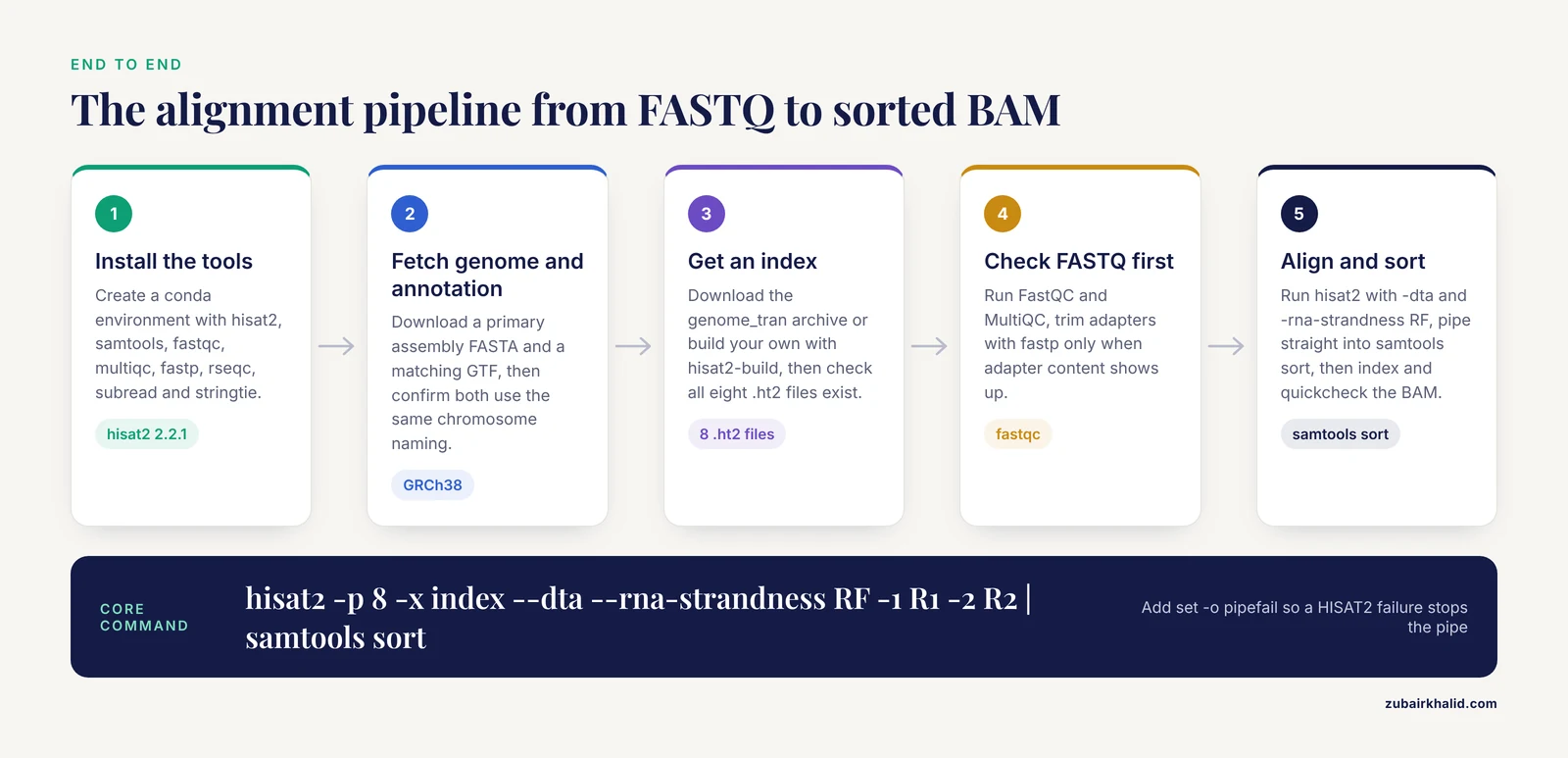
This is the command this tutorial builds toward, for one paired-end sample against the prebuilt GRCh38 transcriptome index:

hisat2 -p 8 -x index/GRCh38.genome_tran/GRCh38.genome_tran \
  --dta \
  --rna-strandness RF \
  --rg-id WT_rep1 --rg SM:WT_rep1 --rg PL:ILLUMINA \
  -1 trimmed/WT_rep1_R1.fastq.gz \
  -2 trimmed/WT_rep1_R2.fastq.gz \
  --no-unal \
  --summary-file logs/WT_rep1.hisat2.summary \
  2> logs/WT_rep1.hisat2.log \
| samtools sort -@ 8 -o bam/WT_rep1.bam -

Before running a full study, test the whole chain on a subsample. Four hundred thousand pairs is enough to exercise every flag:

zcat fastq/WT_rep1_R1.fastq.gz | head -n 800000 | gzip > test_R1.fq.gz
zcat fastq/WT_rep1_R2.fastq.gz | head -n 800000 | gzip > test_R2.fq.gz

What Each Flag Does

• -x points at the index prefix. This is the single most common source of errors, so verify the path and the basename against the .ht2 files on disk.
• -p 8 uses eight threads. Match this to the cores you actually have.
• -dta (downstream transcriptome assembly) tailors the output for assemblers such as StringTie. It restricts reporting to primary alignments and adds the XS strand tag to spliced alignments. Use it whenever transcript assembly is on your roadmap, because adding it later means realigning everything.
• -rna-strandness RF declares the library orientation. RF means read 1 corresponds to the complement of the RNA strand and read 2 to the RNA strand, which is the behavior of dUTP-based stranded kits in paired-end mode. For single-end dUTP data use R. For unstranded libraries, omit the option entirely. Section Step 8 shows how to verify this empirically.
• -rg-id and -rg attach read group tags (sample metadata embedded in the BAM). featureCounts, Picard, and most pipelines use these to track which BAM came from which sample, so set them from the start.
• -no-unal suppresses unaligned reads in the output, which cuts BAM size with no loss for quantification workflows.
• -summary-file writes the alignment summary to a machine-readable file, which MultiQC can aggregate across samples.
• 2> captures the stderr log, which contains the same summary plus any warnings.
• The pipe into samtools sort converts SAM to a coordinate-sorted BAM in one step, so no intermediate SAM file ever touches the disk. Add set -o pipefail at the top of your script so a HISAT2 failure inside the pipe stops the pipeline instead of leaving you an empty BAM.

Reading the Alignment Summary

HISAT2 prints a summary to stderr and to the summary file. An abbreviated, representative example for a 25-million-pair library:

HISAT2 summary stats on this set of alignments:
	Total pairs: 25000000
		Read 1: 25000000
		Read 2: 25000000
	Total paired: 23000000 (92.00%)
		Aligned pair (0 discordant): 22500000 (90.00%)
		Aligned pair (1 discordant): 500000 (2.00%)
	Total unpaired: 4000000 (8.00%)
		Aligned 0 time: 2800000 (70.00%, of unpaired)
		Aligned 1 time: 1000000 (25.00%, of unpaired)
		Aligned >1 times: 200000 (5.00%, of unpaired)
	Overall alignment rate: 94.40%

The final line, Overall alignment rate, is the headline number: the percentage of all reads (both mates) that aligned somewhere. Well-prepared mammalian RNA-seq libraries commonly land between roughly 75 and 95 percent. Rates in the 50s or below usually mean something fixable is wrong: the wrong reference species, the wrong genome build, heavy rRNA or adapter contamination, or corrupted FASTQ files. High rates do not by themselves prove the alignment is correct, which is why the quality control section exists.

Step 6: Sort, Index, and Verify the BAM

The pipe in Step 5 already produced a coordinate-sorted BAM. Index it so genome browsers and downstream tools can access it randomly:

samtools index bam/WT_rep1.bam
samtools quickcheck bam/WT_rep1.bam && echo OK
samtools flagstat bam/WT_rep1.bam
samtools idxstats bam/WT_rep1.bam | head

Representative, abbreviated flagstat output for the library above:

47200000 + 0 in total (94.40% : 0.00% duplicates)
47200000 + 0 mapped (94.40% : 0.00% duplicates)
50000000 + 0 paired in sequencing
25000000 + 0 read1
25000000 + 0 read2
45000000 + 0 properly paired (90.00%)
...

The idxstats output lists each reference sequence with mapped and unmapped counts, which doubles as a chromosome naming check from Step 2.

A 25-million-pair BAM lands in the range of a few gigabytes. For long-term storage, CRAM files (a compressed BAM equivalent that references the original FASTA) save substantial space:

samtools view -C -T reference/GRCh38.fa bam/WT_rep1.bam > bam/WT_rep1.cram

Keep BAMs for active work and convert to CRAM when a project moves to cold storage.

Step 7: Align a Whole Study in One Loop

Real studies process many libraries with identical settings. Published bulk RNA-seq projects routinely handle dozens of libraries, such as a tea flower study that prepared RNA-seq and small RNA-seq libraries from the same 21 biological samples across seven dissected tissues [2]. A shell loop keeps every parameter identical across samples, which is what differential expression analysis assumes.

set -o pipefail
mkdir -p bam logs
for sample in WT_rep1 WT_rep2 WT_rep3 KO_rep1 KO_rep2 KO_rep3
do
  hisat2 -p 8 -x index/GRCh38.genome_tran/GRCh38.genome_tran \
    --dta \
    --rna-strandness RF \
    --rg-id ${sample} --rg SM:${sample} --rg PL:ILLUMINA \
    -1 trimmed/${sample}_R1.fastq.gz \
    -2 trimmed/${sample}_R2.fastq.gz \
    --no-unal \
    --summary-file logs/${sample}.hisat2.summary \
    2> logs/${sample}.hisat2.log \
  | samtools sort -@ 8 -o bam/${sample}.bam -
  samtools index bam/${sample}.bam
done
multiqc logs qc -o qc/multiqc

For a six-sample project at 25 million pairs each, expect roughly 15 to 25 GB of BAM files plus the FASTQ inputs. For a 21-library project, double that again. GNU parallel is a good alternative to the loop when you have many samples and want to run several alignments at once.

Step 8: Get Strandedness Right

Strandedness (also called library orientation) describes which read of a pair follows the direction of the transcript. HISAT2 accepts four values for -rna-strandness: F (the read, or read 1, follows the RNA strand), R (the read, or read 1, follows the complement), FR (read 1 follows the RNA strand, read 2 the complement), and RF (read 1 the complement, read 2 the RNA strand).

Strandedness matters because it changes which overlapping features a read can be assigned to. Genes overlap on opposite strands far more often than people expect, and reads from antisense transcription exist. Getting orientation wrong misassigns counts and can silently halve them for overlapping loci. Strand-specific libraries also enable strand-aware discovery, as in a wheat study that used strand-specific RNA-seq data to identify thousands of intergenic long non-coding RNAs, where assigning the transcribed strand is part of the discovery itself [3].

Most dUTP-based stranded kits behave as RF in paired-end mode and R in single-end mode, but kit behavior varies and documentation is not always explicit. Verify empirically with RSeQC's infer_experiment.py, which compares read orientation against annotated gene models (RSeQC publishes reference BED files for common genomes):

infer_experiment.py -r hg38_RefSeq.bed -i bam/WT_rep1.bam

Illustrative output for a stranded paired-end library:

This is PairEnd Data
Frac. of read-1 mapped to '+': 0.04
Frac. of read-1 mapped to '-': 0.46
Frac. of read-2 mapped to '+': 0.46
Frac. of read-2 mapped to '-': 0.04

The interpretation rule is simple. In an unstranded library the fractions hover near 0.5 across categories. In a stranded library one orientation dominates. If read 2 agrees with the annotated transcript strand most of the time, as in the example above, the library behaves as RF. If read 1 agrees most of the time, it behaves as FR. Run this on one sample from each library type before you commit the whole study to a strandness setting.

Step 9: Splice Junction Options Worth Knowing

The prebuilt genome_tran indexes already embed splice sites, and the custom build in Step 3 embeds them through the -ss and -exon options. Three runtime options refine junction handling.

• -known-splicesite-infile <file> supplies a list of known junctions at alignment time. Point it at the splice_sites.txt file from Step 3 when you aligned against a plain index but have a good annotation.
• -max-intronlen caps the intron length HISAT2 will consider, with a default of 500,000 bases tuned for mammalian genomes. For organisms with short introns, such as many fungi where introns are typically well under a thousand bases, a cap in the low thousands prevents spurious long-range spliced alignments.
• -novel-splicesite-outfile <file> writes the junctions HISAT2 discovered that were not in the known set. Collecting these across all samples is the standard route to annotating novel junctions, though junction discovery needs depth. Twenty to thirty million paired reads covers well-annotated genes, while rare isoforms and low-expression junctions need more.

Recent HISAT2 releases (2.2.0 and later) also offer -tmo, transcriptome mapping only, which restricts output to reads mapping the transcriptome and shrinks BAM files. Skip it if you want the full genomic alignment picture for quality control, since it removes the background alignments that QC metrics partly rely on.

Error Messages You Will Actually See

• Could not locate a HISAT2 index starting with 'grch38_tran'. The -x path or basename does not match the files on disk. Run ls index//.ht2, take the shared prefix up to .1.ht2, and pass exactly that.
• A halt complaining that read 1 and read 2 names disagree, printing the two offending read identifiers. The R1 and R2 files are out of order or from different samples. Re-pair them with a tool such as fastq-pair or re-download matched files. Never align shuffled mates, since every pair-level statistic becomes meaningless.
• [E::hts_open_format] Failed to open file ... from samtools. The output directory does not exist or the path has a typo. Create it with mkdir -p and check the path.
• A memory allocation failure from samtools sort. The machine ran out of RAM. Lower the per-thread memory with -m 2G, reduce threads, or move to a larger machine.
• unexpected end of file from zcat or HISAT2 while reading a FASTQ. The gzip file is truncated, usually from an interrupted transfer. Run gunzip -t file.fastq.gz to test, check checksums against the source, and re-download.

Quality Control: Checking That the Alignment Worked

Alignment rate is the first gate, not the last. Three RSeQC diagnostics catch the problems that rates miss. All of them take a gene model BED file, which RSeQC provides prebuilt for common genomes.

geneBody_coverage.py -i bam/ -r hg38_RefSeq.bed -o qc/genebody
read_distribution.py -r hg38_RefSeq.bed -i bam/WT_rep1.bam
junction_saturation.py -r hg38_RefSeq.bed -i bam/WT_rep1.bam -o qc/junc/WT_rep1

geneBody_coverage plots read density across the scaled length of transcripts. A roughly uniform profile is healthy. A strong skew toward the 3-prime end indicates degraded RNA or a biased library, and it will distort differential expression before you see a single p-value. read_distribution reports the fraction of reads landing in exons, introns, and intergenic regions, and it flags rRNA contamination when a large share of reads sits outside annotated exons in repetitive regions. junction_saturation plots junction discovery against read depth, and a curve that has not plateaued tells you more reads would find more junctions.

Aggregate everything with MultiQC, which parses HISAT2 summary logs, FastQC, fastp, samtools stats, and RSeQC output into one report:

multiqc logs qc -o qc/multiqc

A healthy sample shows a high overall alignment rate, mostly exonic reads for a polyA mammalian library, uniform gene body coverage, a duplicate rate consistent with the input amount, and a strandedness result that matches the kit. When a sample deviates, compare it against its replicates before blaming the biology.

From Aligned Reads to Counts and Differential Expression

For gene-level differential expression, count reads per gene with featureCounts from the subread package:

mkdir -p counts
featureCounts -T 8 -p --countReadPairs -s 2 \
  -t exon -g gene_id \
  -a reference/genes.gtf \
  -o counts/all_samples.txt bam/*.bam

The -s setting must match your library: 2 for reverse-stranded dUTP libraries (the common Illumina stranded case), 1 for forward-stranded, 0 for unstranded. The -countReadPairs flag requires subread 2.0 or later. The resulting count matrix feeds DESeq2 or edgeR for differential expression.

For transcript-level work, assemble with StringTie, which is why the alignments were made with -dta:

stringtie bam/WT_rep1.bam -G reference/genes.gtf -p 8 -o stringtie/WT_rep1.gtf
stringtie --merge -G reference/genes.gtf -o stringtie/merged.gtf stringtie/mergelist.txt

This is the point where the biology starts. Published RNA-seq studies take the count matrix into differential expression, Gene Ontology and KEGG pathway enrichment, and co-expression network analysis, as in an insect study comparing mass-reared and wild strains [4], a chicken study that tied transcriptome changes to infection time points and pathology [5], and a rice study that combined RNA-seq co-expression networks with haplotype analysis and qRT-PCR validation to prioritize a salinity-tolerance candidate gene [6]. Aligned BAMs also feed integrative designs: bladder cancer biomarker work combined bulk RNA-seq with single-cell and proteomic datasets to prioritize candidate genes [7], cervical cancer prognostic modeling integrated bulk transcriptomic data with single-cell profiles [8], a gastric cancer study built survival risk scores from bulk cohort data and linked them to stromal features [9], and a mouse mammary tumor study used bulk transcriptomics to connect genetic background with immune recognition of tumors [10].

One habit protects all of that downstream work. Record the exact tool versions, index build, annotation release, and every flag in a log or a version-controlled script. When raw data get reanalyzed later, as in a Leishmania meta-analysis that reprocessed public RNA-seq data through a unified pipeline with standardized quality control, differential expression, and batch-effect correction, the reproducibility of the original alignment parameters is what makes cross-study comparison defensible [11].

For visualization, generate normalized genome browser tracks from the BAMs with deepTools:

bamCoverage -b bam/WT_rep1.bam -o qc/bigwig/WT_rep1.bw --normalizeUsing CPM -p 8

Load the bigWig files plus the BAM and its index in IGV, click through to a housekeeping gene, and confirm that reads pile up across exons and span introns with junction reads. Ten minutes of eyeballing catches sample swaps and strand disasters that summary statistics hide.

Key HISAT2 Options at a Glance

Common Mistakes and Limitations

1. Mismatched genome build or chromosome naming. Aligning against GRCh38 with a GRCh37 annotation, or against an index named 1 with a GTF named chr1, produces alignments that look fine and counts that are quietly wrong. Keep FASTA, GTF, and index from one source, and confirm names with samtools idxstats.
2. Guessing strandedness instead of measuring it. A wrong -rna-strandness value combined with the wrong featureCounts -s value misassigns or discards counts at overlapping loci. Run infer_experiment.py on one sample per library type before committing.
3. Forgetting -dta before transcript assembly. Without it, spliced alignments lack the XS strand tag and reporting is not assembler-friendly, so StringTie loses or mislabels junctions. Decide the downstream path before aligning, because changing it means realigning.
4. Treating the alignment rate as the whole QC story. A sample can align at 90 percent and still be ruined by 3-prime degradation, rRNA contamination, or a sample swap. geneBody_coverage, read_distribution, and replicate correlation catch what the rate cannot.
5. Over-trimming reads. Aggressive quality clipping shortens reads, and short reads cannot anchor confidently across splice junctions. Remove adapters when detected, leave the rest of the read alone for modern data.
6. Expecting HISAT2 to quantify anything. HISAT2 produces alignments. Gene counts come from featureCounts or htseq-count, transcript estimates from StringTie or Salmon. Budget time for those steps explicitly.
7. Using HISAT2 for the wrong library type. Small RNA-seq reads are short, unspliced, and better served by dedicated microRNA pipelines, as in studies that profile small RNA libraries alongside standard mRNA libraries from the same samples [2]. Single-cell RNA-seq needs purpose-built pipelines with cell barcodes and UMI handling, learned best through guided annotated workflows [1].
8. Skipping sort and index. An unsorted BAM cannot be indexed, cannot be viewed in IGV, and slows or breaks downstream tools. The pipe into samtools sort in this tutorial handles it, but only if you keep it in your own scripts.
9. Ignoring reproducibility. Six months later, nobody remembers which annotation release or flags produced a BAM. Save the script, the conda environment export, the index source, and the HISAT2 version with the results, because standardized, documented pipelines are what make later reanalysis and meta-analysis possible [11].
10. Knowing the limits of the aligner. Reads from pseudogene-rich regions multimap and get ambiguous assignments, which is a property of the human genome rather than a HISAT2 defect. Novel junction detection depends on depth, so absence of a junction in shallow data is not evidence of absence in the transcriptome. And HISAT2 trades some raw speed for its low memory footprint, so extremely large cohorts on beefy hardware sometimes prefer STAR, while pure quantification projects without junction discovery needs often prefer Salmon.

Frequently Asked Questions

How many reads per sample do I need for RNA-seq alignment with HISAT2?

Twenty to thirty million paired-end reads is a common target for gene-level differential expression in mammalian samples, and considerably more for isoform or novel splice junction discovery, where rare transcripts need depth.

Should I trim adapters before aligning with HISAT2?

Yes, if FastQC shows adapter content, run fastp with adapter detection first. Otherwise skip trimming, because aggressive quality clipping shortens reads and weakens splice junction anchoring.

What is a good overall alignment rate for HISAT2?

Well-prepared mammalian RNA-seq libraries commonly land between roughly 75 and 95 percent. Values in the 50s or below usually indicate the wrong reference, contamination, or corrupted files and deserve investigation before proceeding.

Should I use HISAT2, STAR, or Salmon for my RNA-seq project?

Use HISAT2 when you want full splice-aware alignment with a low memory footprint, STAR when you have tens of gigabytes of RAM and want maximum speed, and Salmon when you only need transcript quantification and do not need a BAM for browser inspection or junction discovery.

How do I choose the right strandness setting in HISAT2?

Check your library kit documentation first, then verify empirically with RSeQC infer_experiment.py on one sample. Most paired-end dUTP kits behave as RF, most single-end dUTP kits as R, and unstranded libraries should omit the option entirely.

Can HISAT2 read gzipped FASTQ files directly?

Yes, HISAT2 reads gzip-compressed FASTQ without any preprocessing, so you can pass .fastq.gz files directly to -1 and -2 and avoid decompressing large files.

What does the dta flag do and when do I need it?

The dta flag tailors output for transcript assemblers by reporting primary alignments and adding the XS strand tag to spliced reads. Use it whenever StringTie is in your plans, because adding it later requires realigning every sample.

Can I use HISAT2 for single-cell RNA-seq data?

No, single-cell data need pipelines that handle cell barcodes and UMIs, such as STARsolo or alevin-fry. HISAT2 is built for bulk RNA-seq, and single-cell analysis is best learned through dedicated guided workflows.

Sources

1. Using In Silico Pseudobulk Differential Expression and Trajectory Analysis of Single Cell RNA Sequencing to Reveal Stem Cell State Transitions in Colonic Inflammation.
2. Integrated RNA-seq and small RNA-seq profiling reveals tissue-associated transcriptional programs and candidate miRNA-mRNA relationships across tea floral tissues.
3. Identification and expression analysis of intergenic long non-coding RNAs (lincRNA) associated with stripe rust resistance in wheat.
4. Comparative transcriptomic analysis of functional and metabolic changes in mass-reared and wild Anastrepha ludens Loew (Diptera: Tephritidae).
5. Transcriptomic analysis of cecal mucosal immunity in SPF White Leghorn chicks infected with precocious and parent strains of Eimeria tenella.
6. QTL mapping and haplotype analysis reveal candidate genes for seedling-stage salinity tolerance in rice.
7. Integrative Multi-Omics Analysis with Interpretable Machine Learning Prioritizes Candidate Biomarkers for Bladder Cancer.
8. Transcriptomics and single-cell RNA sequencing uncover prognostic characteristics and immune regulatory mechanisms of lactylation in cervical cancer.
9. Integrated Single-cell and Bulk Transcriptomic Analysis Links NOTCH Signaling to Stromal Features and Prognosis in Gastric Cancer.
10. Early-onset spontaneous murine mammary tumors show increased lymphocyte representation and reduced MHC antigen presentation.
11. Integrative transcriptomics and hypothesis-driven transfer machine learning reveal conserved and species-specific host-parasite dynamics across Leishmania species in THP-1 cells: a systematic review and meta-analysis.