Gviz vs karyoploteR: Which R Package Should You Use
By Dr. Zubair Khalid, DVM, MS, PhD ·

Gviz draws a single genomic locus as a stack of horizontal tracks, while karyoploteR draws data across whole chromosomes or an entire karyotype. If you need a publication figure of one gene region with genes, sequence, and a coverage track, use Gviz. If you need to see how a signal or a set of variants is distributed across the whole genome, use karyoploteR. Many mature projects end up using both, one for zooming in and one for zooming out.
This guide is a practical comparison written for people doing R for bioinformatics. It explains what each package is built for, how the two architectures differ, which criteria actually decide the choice in real projects, and worked scenarios where one package is clearly the better fit. It also doubles as a compact Bioconductor tutorial reference, since both packages live in the Bioconductor ecosystem and speak the same underlying data language of GenomicRanges objects.
Quick Answer and Side-by-Side Comparison
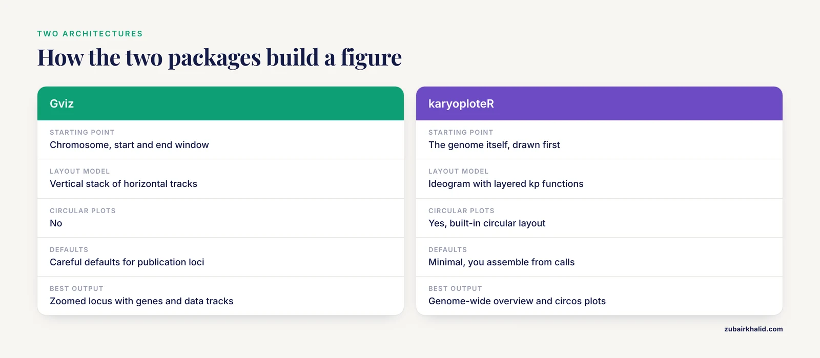
The core difference between Gviz and karyoploteR is the coordinate system they assume. Gviz is locus-centric: you give it a chromosome, a start, and an end, and it assembles annotation and data into vertical track lanes that all share that window [1]. karyoploteR is genome-centric: it first draws the chromosomes themselves, then provides plotting functions that place your data onto those chromosomes, either linearly or in circular layouts.
Both packages accept genomic data represented as GRanges objects, which are Bioconductor's standard container for intervals on a genome. That shared foundation means your upstream data wrangling, done with tools like GenomicRanges and rtracklayer, is reusable regardless of which plotting package you choose.
| Criterion | Gviz | karyoploteR |
|---|---|---|
| Primary scale | Single locus, from hundreds of bases up to roughly a few megabases | Whole chromosomes, whole genomes, sets of chromosomes |
| Layout model | Vertical stack of horizontal tracks | Karyotype ideogram with layered plotting functions |
| Circular plots | No | Yes, built-in circular layout |
| Built-in data retrieval | Direct access to Ensembl (through biomaRt) and UCSC, plus standard file formats [1] | Genome definitions from BSGenome, TxDb, or your own GRanges, data supplied by you |
| Annotation file support | Common annotation types including GFF/GTF, BED, and BAM [1] | Reads GRanges and related Bioconductor objects, converters exist upstream |
| Alignment data | AlignmentTrack renders read-level BAM data | kpPlotBAMCoverage for coverage, not read-level detail |
| Default behavior | Careful defaults designed for publication-ready loci figures [1] | Minimal defaults, you assemble the figure from function calls |
| Customization style | displayPars on track objects | Base-R-style layering, one function per graphical element |
| Non-model organisms | Workable, but annotations are easiest for well-annotated genomes | Straightforward, any genome defined as GRanges works |
| Learning curve | Moderate, mostly about learning track types | Moderate, mostly about learning the kp function family |
| Best output | Zoomed-in locus figure with genes, axis, ideogram, and data tracks | Genome-wide overview, chromosome-level distributions, circos-style plots |
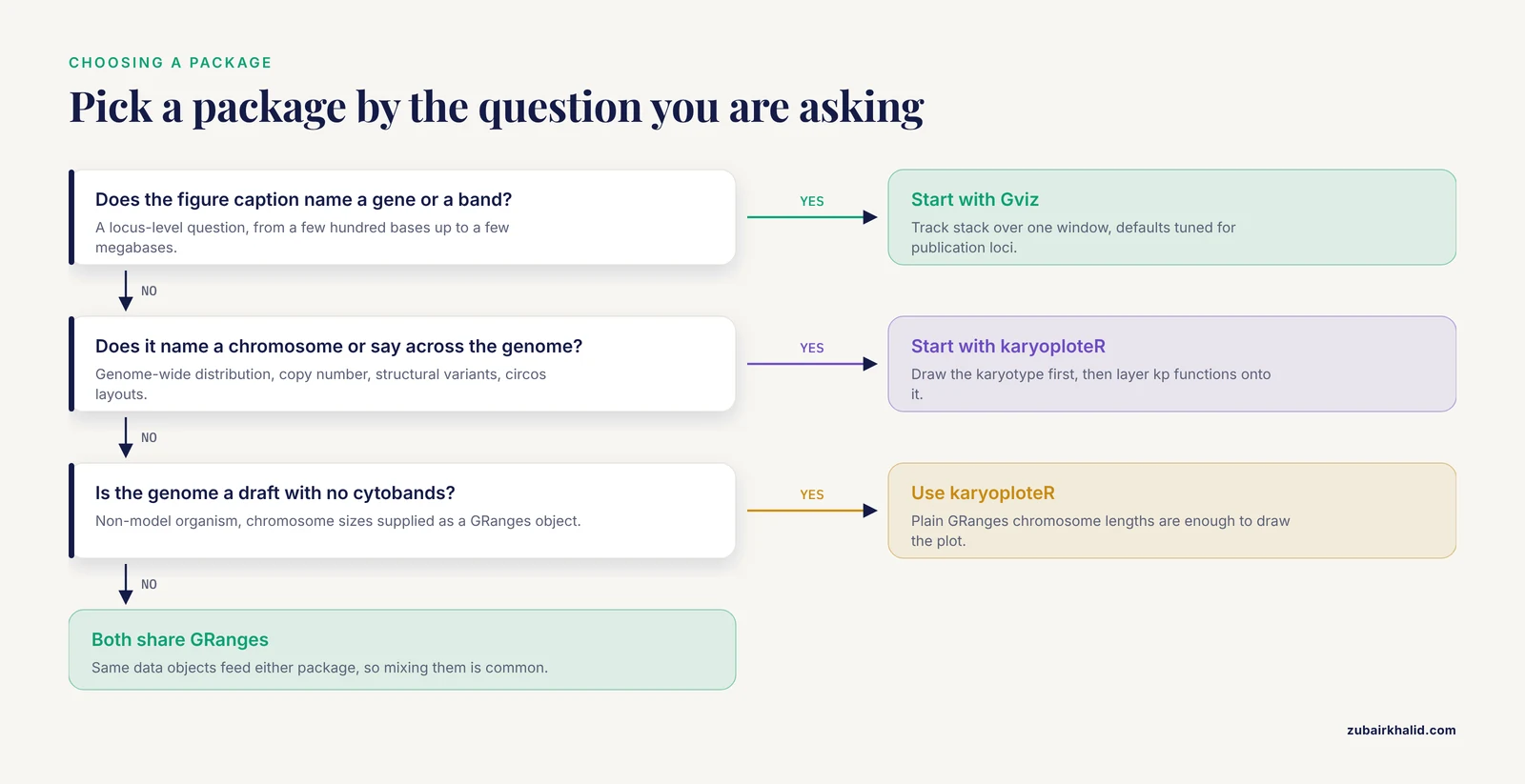
A one-line rule of thumb: if your figure caption names a chromosomal band or a gene, reach for Gviz first. If your figure caption names a chromosome or says "across the genome," reach for karyoploteR first.
What Gviz Is and When to Use It
The track-based architecture
Gviz was built around a simple observation: almost every genomic locus figure in the literature has the same anatomy. There is an ideogram strip showing where you are on the chromosome, a genome axis with base-pair coordinates, a gene or transcript track, and one or more data tracks showing coverage, read density, variant positions, or methylation values. Gviz formalizes each of these as a track object, and the plotTracks function renders a list of tracks in a single aligned stack.
The track types cover the common cases:
- IdeogramTrack draws the cytoband ideogram for the chromosome you are viewing.
- GenomeAxisTrack draws the base-pair ruler.
- AnnotationTrack places intervals such as BED features or ChIP peaks.
- GeneRegionTrack draws gene and transcript models with exons, introns, and UTRs.
- DataTrack draws quantitative data per position or per interval, with plotting styles that include lines, area fills, histograms, heatmaps, and horizons.
- SequenceTrack renders the actual nucleotide sequence when the window is small.
- AlignmentTrack renders BAM alignment files down to individual reads, including mismatch coloring.
- OverlayTrack lets you stack several data sources into one lane.
Because each track is an object with its own display parameters, you tweak a figure by adjusting displayPars on individual tracks rather than rebuilding the plot. Gviz ships with carefully chosen defaults so that a first pass with plotTracks often produces a figure close to publication quality, which the package documentation and its methods paper both emphasize as a design goal [1].
When to use Gviz
Reach for Gviz when the question is local. Typical cases include:
- Showing sequencing coverage, splice junctions, or variant calls across one gene or one candidate region.
- Comparing RNA-seq signal between conditions at a specific transcript.
- Displaying ChIP-seq or ATAC-seq peaks together with gene models for a promoter of interest.
- Inspecting a variant callset in context, for example a single exome-derived SNV sitting inside an exon.
- Producing the standard "browser shot" figure for a paper, where reviewers expect gene models, an axis, and one or two data tracks over a few hundred kilobases.
Gviz is also the natural choice when you want it to fetch the annotation for you. It connects directly to external sources such as Ensembl and UCSC, so you can request a gene region track for a chromosome window and let the package pull transcript models rather than downloading GTF files yourself [1]. For a quick exploratory look, this removes an entire data-management step. For a fully reproducible pipeline, you can still supply local GTF files, which is usually the better practice because remote resources change over time.
A minimal working example
The following example draws a coverage track and gene models around the TP53 locus on chromosome 17 using hg38 coordinates. The TP53 gene spans roughly chr17:7,668,421 to 7,687,483 in GRCh38, a 19-kilobase window that is well within Gviz's comfort zone.
library(Gviz)
library(TxDb.Hsapiens.UCSC.hg38.knownGene)

chr  <- "chr17"
from <- 7668421
to   <- 7687483

itrack <- IdeogramTrack(genome = "hg38", chromosome = chr)
axtrack <- GenomeAxisTrack()
gtrack <- GeneRegionTrack(TxDb.Hsapiens.UCSC.hg38.knownGene,
                          genome = "hg38", chromosome = chr,
                          name = "Genes")
dtrack <- DataTrack(range = my_coverage_granges,
                    genome = "hg38", chromosome = chr,
                    type = "histogram", name = "Coverage")

plotTracks(list(itrack, axtrack, gtrack, dtrack),
           from = from, to = to)
The key habits to learn are that every track must be told which genome and chromosome it belongs to, that plotTracks accepts a list and aligns all tracks to the same window, and that displayPars controls individual visual settings. Once those three ideas are in place, the rest of the package is pattern repetition.
What karyoploteR Is and When to Use It
The karyotype-first architecture
karyoploteR inverts the Gviz model. Instead of starting with a data window, it starts with the genome itself. The plotKaryotype function draws chromosomes as ideograms, either using cytoband definitions available for standard genomes or, for genomes without band data, simple chromosome rectangles with sensible lengths. Everything after that is additive: the package exposes a large family of kp functions, and each call adds one graphical layer onto the existing karyotype.
The function names map directly to what they draw, which makes scripts readable:
- kpDataBackground shades the data panel behind a chromosome or region.
- kpPoints plots points such as variant positions or association signals.
- kpBars plots bars such as per-window counts.
- kpSegments draws connectors, useful for linking paired features.
- kpHeatmap fills regions with color intensity scales.
- kpPlotRegions fills chromosomal intervals with colored blocks.
- kpPlotBAMCoverage computes and draws read coverage directly from a BAM file.
- kpPlotBigWig draws signal from bigWig files.
- autotrack partitions the plotting space into lanes when you have many track categories.
This is deliberately similar in spirit to base R graphics, where you call plot once and then annotate with points, lines, and text. If you already think in base-R plotting terms, karyoploteR feels familiar within an afternoon.
When to use karyoploteR
Reach for karyoploteR when the question is global. Typical cases include:
- Showing the genome-wide distribution of mutations, for example SNV density per chromosome in an evolution or tumor experiment.
- Displaying copy-number segments or structural variants across every chromosome at once.
- Visualizing GWAS or QTL results genome-wide, with one lane per trait or per population.
- Producing circos-style plots, since plotKaryotype supports a circular layout where chromosomes are arranged as a ring and data can be linked between positions.
- Working with non-model organisms. Because you can supply chromosome sizes as a plain GRanges object, a draft genome with no cytoband data is not a barrier, which makes karyoploteR a common choice outside the standard model species.
The genome-wide view matters for scientific reasoning as much as for figures. In experimental evolution work, for example, a student or researcher needs to see whether adaptive mutations cluster on one chromosome or spread across the genome before deciding which candidate genes deserve closer attention [2]. A per-locus browser view cannot answer that clustering question, but a karyotype plot answers it at a glance.
A minimal working example
This example draws chromosome 1 of hg19 with a shaded data panel and variant positions plotted as points whose vertical position is jittered inside the panel.
library(karyoploteR)

kp <- plotKaryotype(genome = "hg19", chromosomes = "chr1")
kpDataBackground(kp, data.panel = 1)
kpPoints(kp, data = variant_gr, r0 = 0.4, r1 = 0.95,
         pch = 16, cex = 0.6, col = "#1f4e79")
The r0 and r1 arguments control the vertical band inside the data panel where points are placed, and they are the main tool for building multi-layer figures. A circular layout is a one-argument change:
kp <- plotKaryotype(plot.type = "circle")
kpPlotRegions(kp, data = cnv_gr, r0 = 0, r1 = 1)
The mental model to internalize is that every kp function takes the plot object returned by plotKaryotype as its first argument. You keep that object in a variable and progressively decorate it, which is exactly how layered figures get assembled.
The Difference Between Gviz and karyoploteR on the Criteria That Matter
Knowing the architecture of each package is not the same as knowing which one to open first on a deadline. The difference between Gviz and karyoploteR becomes concrete on five criteria: scale, data handling, default versus manual assembly, learning curve shape, and behavior outside standard genomes.
Scale and zoom range
Gviz is designed for windows where individual features are still visually meaningful. Once you ask it to render tens of megabases, gene models compress into sludge and data tracks lose resolution. The package is happiest from a few hundred bases, where SequenceTrack can even render individual nucleotides, up to loci measured in single-digit megabases.
karyoploteR is designed for the opposite end. It renders all chromosomes in one figure by default, and it degrades gracefully when your data are dense, because the karyotype itself, not your data, defines the visual structure. If you try to use karyoploteR for a 50-kilobase locus, you will find yourself fighting the layout, and Gviz will do the job with less effort.
A practical consequence is that these two scales complement each other. A common figure in sequencing papers shows a genome-wide overview panel generated with a karyotype-style plot, then zoomed locus panels underneath it generated in a browser style. Using both packages for that pair of figures keeps the visual language consistent because both understand GenomicRanges inputs.
Data input and Bioconductor integration
Both packages live inside the Bioconductor ecosystem and share its conventions, which is a major practical advantage of doing R for bioinformatics. Gviz is described in its methods paper as tightly embedded in the Bioconductor genomics landscape, integrating with existing infrastructure and supporting most commonly used annotation file types [1]. In practice, this means you can hand it GRanges from your own analysis, point it at a BAM or bigWig file, or load annotation from a TxDb package.
karyoploteR accepts GRanges and related objects for everything data-like, and gets its chromosome definitions from BSGenome packages, TxDb packages, or user-supplied GRanges. It does not fetch annotations from remote services the way Gviz does. That is a difference in philosophy rather than capability: Gviz optimizes for convenient first contact with well-annotated genomes, while karyoploteR optimizes for the case where you already have your data and your genome definition locally.
This is also where modern R toolkits show a common pattern of workflow integration. LDblockR, for example, unifies linkage disequilibrium statistics, regional annotation, and publication-ready regional visualization in a single R-native object model, and its authors identify workflow integration rather than a new statistical estimator as the principal contribution [3]. Whether a tool wraps Gviz-style track rendering or karyoploteR-style regional plotting, the value proposition in the current ecosystem is increasingly about gluing steps together rather than any single plot type.
Defaults versus manual assembly
Gviz's design goal was to make production of publication-ready figures of genomic loci easy through carefully chosen defaults, while keeping high flexibility through customization options [1]. Concretely, this means that plotTracks with sensible track objects usually produces something a journal would accept with only minor styling. You spend your time choosing what to show, not how to lay it out.
karyoploteR gives you almost no defaults beyond the chromosome drawing itself. You decide on backgrounds, lanes, vertical ranges, labels, and colors through explicit function calls. This is slower for a first figure and faster for a tenth figure, because once you have written the layering code once, you adapt it to new data by swapping the GRanges input. The same tradeoff shows up throughout R-based visualization work in genomics, where packages such as ggplot2, dplyr, ggrepel, and tidyr are used to assemble custom publication figures from multi-omics data, accepting more code in exchange for full control [4].
Learning curve shape
The two packages have different frustration profiles. With Gviz, the early learning curve is gentle because defaults carry you, and the friction arrives when you need unusual styling, for example custom grouping of annotation features or fine control over track heights. With karyoploteR, the early curve is steeper because you must assemble everything, but the model is so uniform that expertise compounds quickly, and the documentation's examples transfer directly to new data types.
If you are teaching a course or writing a short Bioconductor tutorial, Gviz tends to produce satisfying results in the first session, while karyoploteR produces satisfying results once students have learned roughly six or seven kp functions. Both packages reward reading their vignettes, which are among the better-maintained in the Bioconductor ecosystem.
Performance and large data
Neither package will render an entire human BAM file read by read, and neither is meant to. For coverage-style summaries, both perform well when you pre-reduce your data into per-window statistics. A useful habit in R for bioinformatics is to bin signal data into fixed windows with GenomicRanges before plotting, which makes Gviz DataTracks and karyoploteR bar or heatmap layers both fast and visually cleaner. For read-level inspection in a narrow window, Gviz's AlignmentTrack is the appropriate tool, and for genome-wide coverage summaries karyoploteR's BAM coverage plotting fits the task.
Worked Scenarios: Gviz or karyoploteR?
Scenario 1: A publication figure of one candidate gene
You have RNA-seq coverage bigWig files for control and treatment, a splice-junction table, and a variant of interest in one exon. The reviewer wants a browser-style figure.
Choose Gviz. Build a DataTrack per condition, an AnnotationTrack or GeneRegionTrack from a local GTF, a GenomeAxisTrack, and an IdeogramTrack, then plotTracks them together over a window spanning the gene plus flanking context. Overlay the two coverage tracks if you want direct comparison in one lane. This is the canonical use case that Gviz's defaults were tuned for [1].
Scenario 2: A genome-wide mutation landscape
You sequenced evolved yeast populations and want to show where mutations landed across all sixteen chromosomes, grouped by population and mutation type.
Choose karyoploteR. Plot the full karyotype, then use autotrack or manual r0 and r1 bands to give each population its own lane, and color-code points by mutation class. This is the kind of question that motivated the yEvo Mutation Browser, which gives students an interactive chromosome map of mutated genes alongside a gene viewer for specific mutation sites [2]. The static karyotype figure and the interactive browser answer different needs, and karyoploteR produces the static, publication-bound version.
Scenario 3: Automated regional plots inside a reproducible pipeline
You maintain a pipeline that processes genotype data and needs consistent regional figures for hundreds of loci, run unattended on a server.
Choose karyoploteR if the regions are chromosome-scale or if you want genome-wide context panels. Choose Gviz if each output is a gene-centered locus figure. Either way, favor programmatic assembly over interactive tweaking. Pipeline-oriented R tools increasingly bake visualization into the same package as the analysis, as seen in LDblockR for regional LD analysis and visualization [3] and in CGAS, an automated comparative chloroplast genomics pipeline whose modules integrate R-based visualizations wherever graphical output is required [5]. The lesson from both is that your plotting layer should accept data objects directly from the analysis layer, which both Gviz and karyoploteR do naturally through GRanges.
Reproducibility across a pipeline also depends on how the surrounding environment is managed. Comparisons of workflow tools have shown that consolidating steps into a single language-native framework reduces friction between raw files, quality-control decisions, and downstream analysis, even when tradeoffs like memory use appear [6]. Keeping plotting inside your R environment rather than shelling out to a separate browser tool is exactly this kind of consolidation.
Scenario 4: An interactive viewer for students or collaborators
You need colleagues or students to explore variant data without writing code.
Neither Gviz nor karyoploteR is interactive. Both render static figures. The standard solution is to wrap your plotting code in an R Shiny application. This is an established pattern: the yEvo Mutation Browser uses R Shiny to deliver an interactive chromosome map, mutation-type graphs, and a gene viewer showing mutation sites within genes [2], and XVCF uses Shiny with packages like vcfR and maftools behind a graphical interface for summarizing and visualizing variant data, including read depth, mapping quality, genotype, and quality-control summaries [7]. In such an app, karyoploteR often serves the chromosome-map panel while Gviz-style logic serves the zoomed gene-view panel, mirroring the split that the yEvo tool implements between its chromosome map and its gene viewer [2].
Scenario 5: Copy number and structural variants across a cancer genome
You have segmented copy-number calls and paired-end structural variant breakpoints and want a single figure communicating the global architecture.
Choose karyoploteR, with plotKaryotype in the circular layout if you want to draw links between breakpoint partners. kpPlotRegions renders the copy-number segments as colored blocks, and kpSegments draws interchromosomal links. Gviz cannot meaningfully render this figure because its model has no concept of two loci on different chromosomes sharing one visual element.
Scenario 6: A non-model organism with a draft assembly
You have a newly assembled genome, a GFF from a pipeline, and variant calls, and no cytoband data anywhere.
Choose karyoploteR. Supply the chromosome names and lengths as a GRanges object to plotKaryotype, and every kp function works immediately. Gviz can also work with custom annotations, but the ideogram and axis components assume more conventional genome setups, and karyoploteR simply asks for less.
Common Mistakes and Limitations
- Using Gviz for genome-wide figures. The most common failure with Gviz is asking it to render a whole chromosome. Gene tracks become illegible and the plot takes a long time to draw. Anything beyond a few megabases should move to a karyotype-style view.
- Using karyoploteR for locus-level detail. karyoploteR does not do base-pair resolution elegantly, has no read-level alignment view, and its axis labeling is not built for examining a 10-kilobase window. Switch to Gviz for those tasks.
- Forgetting to pass the plot object to kp functions. Every karyoploteR plotting function needs the KaryoPlot object as its first argument. A call like kpPoints(gr) without the object errors or, more confusingly, draws onto the wrong plot when multiple plot objects exist.
- Mixing up data.panel. karyoploteR reserves vertical space for data separate from the ideogram. If points appear squashed or invisible, check that r0 and r1 are set inside the correct data panel and that kpDataBackground was called with the same panel value.
- Fetching annotation remotely in scripts that must run later. Gviz's direct Ensembl and UCSC retrieval is convenient for exploration [1], but remote resources change. For any analysis that must be rerun months later, download annotation files locally and load them from disk.
- Treating these packages as interactive genome browsers. They produce static figures. If the requirement is truly interactive exploration, build a Shiny app around them or use an existing browser tool, following the pattern of tools like the yEvo Mutation Browser and XVCF [2].
- Ignoring upstream data hygiene. Both packages plot exactly what you hand them. Overlapping ranges, inconsistent chromosome naming such as chr1 versus 1, and strand confusion produce misleading figures silently. Normalize chromosome naming and sort ranges before plotting.
- Overloading a single figure. A karyotype with nine layers of lanes and three color encodings communicates less than a karyotype with two. Genome-wide plots tempt dense layouts. Plan the layers before writing code.
Frequently Asked Questions
Can Gviz and karyoploteR be used together in one project?
Yes, and it is common. Both speak GRanges, so the same data objects feed either package. Use karyoploteR for the genome-wide overview figure and Gviz for the zoomed locus figures that accompany it, keeping chromosome naming consistent between the two.
Which package handles large datasets better?
Neither is built for read-level rendering at scale. For genome-wide coverage summaries, karyoploteR handles chromosome-scale density plots well, and pre-binning your data into per-window statistics makes both packages fast and readable.
Do these packages require an internet connection?
Gviz can fetch annotation from Ensembl and UCSC directly, which needs connectivity [1], but it also accepts local files. karyoploteR works fully offline as long as you supply genome definitions and data locally, which makes it the safer choice for servers without external access.
Can either package make interactive plots?
No, both produce static figures intended for reports and publications. For interactive exploration, wrap your plotting code in an R Shiny application, the approach used by tools such as the yEvo Mutation Browser and XVCF [2].
Which package should I learn first if I am new to R for bioinformatics?
Learn Gviz first if your work centers on candidate genes and locus figures, because its defaults produce good results early. Learn karyoploteR first if your work centers on genome-wide surveys or non-model organisms. Either way, learn GenomicRanges alongside, since both packages build on it.
Do both packages work for non-model organism genomes?
karyoploteR handles custom genomes with minimal effort because chromosome definitions can be supplied as a plain GRanges object. Gviz also works with custom annotation, but its ideogram and remote retrieval features are most convenient for well-annotated standard genomes.
Sources
- Visualizing Genomic Data Using Gviz and Bioconductor.
- The yEvo Mutation Browser: Enhancing student understanding of experimental evolution and genomics through interactive data visualization.
- LDblockR: a cross-platform R toolkit for multi-format linkage disequilibrium analysis and integrated regional genomics visualization.
- Synergistic role of molecular imaging and genomics in thyroid cancer management: from diagnosis to personalized treatment.
- CGAS (Chloroplast Genome Analysis Suite): An automated python pipeline for comprehensive comparative chloroplast genomics.
- SNPio: a Python interface for population genomic data processing.
- XVCF: Exquisite visualization of VCF data from genomic experiments.