GEO vs. SRA: Which NCBI Database Should You Use for RNA-Seq Data?
By Dr. Zubair Khalid, DVM, MS, PhD ·

GEO stores processed RNA-seq results such as gene count matrices and sample metadata, while SRA stores the raw sequencing reads that produced those results. A simple rule covers most decisions: start at GEO when you want expression tables, study design, and fast reanalysis, and go to SRA when you need the reads themselves to run your own pipeline.
Both repositories belong to NCBI, both appear in the same papers, and both are free. The confusion is understandable because most RNA-seq studies are split across the two. A typical deposit puts raw reads in SRA and processed expression values in GEO, with cross-links between them. A bovine endometrium study under accession GSE65117 is a clean example, with all read sequences deposited in SRA and the gene expression overview deposited in GEO, a dual deposit the authors described as supporting reproducibility and new discovery [1].
This article works as a practical NCBI databases guide for RNA-seq work. It explains what each repository holds, compares them side by side, maps real analysis goals to the right database, and walks through download commands and worked scenarios.
What GEO and SRA Actually Are
GEO: the Gene Expression Omnibus
GEO is NCBI's public archive for functional genomics data, and it is built around processed results rather than raw signal. For microarrays, GEO holds intensity tables. For RNA-seq, it holds derived quantities: count matrices (tables with genes as rows and samples as columns holding the number of reads assigned to each gene), normalized values such as TPM (transcripts per million, a scaled expression unit), sample annotations, and the written description of the experiment.
Three accession types organize everything. A Series (GSE) is one experiment or study, such as GSE65117. A Sample (GSM) is one sequenced library with its own metadata page. A Platform (GPL) describes the measurement technology, which matters more for microarrays than for RNA-seq.
NCBI's submission policy sends raw reads to SRA rather than GEO. A GEO series for RNA-seq therefore contains processed files and links, and the reads live one click away in SRA. This division is deliberate. Counts and metadata are small, standardized, and immediately useful, while raw reads are large and better served by a dedicated read archive.
SRA: the Sequence Read Archive
SRA is NCBI's archive of raw sequencing reads and the technical metadata that describes them. It is the United States node of the International Nucleotide Sequence Database Collaboration, alongside ENA in Europe and DDBJ in Japan, and records are shared across the three.
SRA organizes data in a hierarchy. A Run (SRR) is the output of one sequencing reaction and is the unit you actually download. Runs belong to Experiments (SRX), which describe library preparation and sequencing settings. Experiments belong to Samples (SRS), which belong to Studies (SRP). Two cross-cutting identifiers tie SRA to the rest of NCBI: BioProject (PRJNA) for the study umbrella and BioSample (SAMN) for the biological specimen.
Files arrive as compressed SRA binary format. The sra-tools software converts them to FASTQ, the standard text format that stores sequences and per-base quality scores. Alignments are sometimes deposited as BAM, but FASTQ is the norm. Expect multi-gigabyte files per sample once converted, which is the practical price of working from raw data.
How the Two Repositories Connect
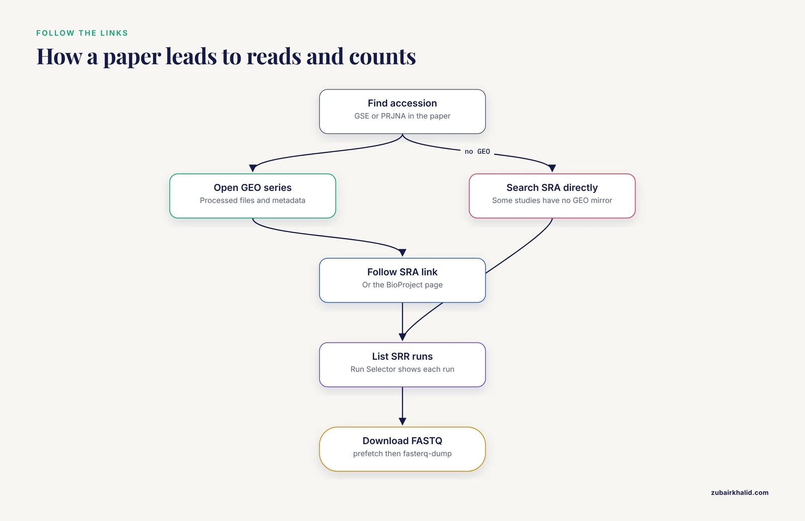
Most modern RNA-seq deposits exist in both places with explicit cross-links. Follow a real chain to see the pattern. A single-nucleus RNA-seq study of human salivary glands is reachable through GEO accession GSE176155, and the same study carries BioProject accession PRJNA735197, which leads to the raw FASTQ files in SRA [2]. A study of opioid use disorder cites its data under PRJNA492904 and pulls the RNA-seq reads from SRA for variant detection [3].
The chain from a paper to reads usually looks like this: find the GSE in the paper, open the GEO series page, follow the SRA or BioProject link, note the SRR run accessions, and download with sra-tools.
Two exceptions keep this from being automatic. Some GEO series have no raw reads behind them, and some SRA studies have no GEO mirror at all. The All of gene Expression (AOE) index was built partly because RNA-seq datasets exist in SRA that never reached GEO or ArrayExpress [4].
GEO vs. SRA for RNA-Seq Data: Side-by-Side Comparison
The difference between GEO and SRA for RNA-seq data comes down to processing level and purpose. The table below puts the structural differences in one place, and the sections after it explain what those differences mean for your analysis.
| Criterion | GEO | SRA |
|---|---|---|
| Core content | Processed expression data, sample metadata, links to raw reads | Raw sequencing reads and per-run technical metadata |
| Typical RNA-seq files | Count matrices, normalized tables, series matrix, supplementary files | SRA binary files convertible to FASTQ, occasionally BAM alignments |
| Organization | Series (GSE), Samples (GSM), Platforms (GPL) | Studies (SRP), Experiments (SRX), Samples (SRS), Runs (SRR) |
| Linked identifiers | BioProject, BioSample, SRA studies | BioProject, BioSample, linked GEO series when one exists |
| Metadata strength | Rich experimental design and per-sample characteristics | Per-run instrument, layout, read length, library strategy |
| Download burden | Kilobytes to megabytes per sample | Multi-gigabyte files per sample |
| Best for | Reanalysis of counts, meta-analysis, machine learning on expression | Custom alignment, variant calling, reprocessing, QC audits |
| Analysis stage | Downstream | Upstream |
| Coverage caveat | Some RNA-seq is never deposited here | Near-complete read archive, but not every study has a GEO mirror |
Neither database is the winner in the abstract. GEO wins on speed and convenience, SRA wins on control and completeness, and most serious projects use both.
When to Use GEO
You Need a Count Matrix Today
Processed data is GEO's core product. Supplementary files on a series page often include raw gene counts, normalized matrices, and per-sample annotation tables, all downloadable in seconds. The GREIN web platform (GEO RNA-seq Experiments Interactive Navigator, at shiny.ilincs.org/grein) goes further, offering more than 6,500 GEO RNA-seq datasets already processed through a uniform back-end pipeline, with interactive visualization, subsetting, statistical power analysis, differential expression signature construction, and download of processed tables [5]. If your question fits inside the submitted design, this is the fastest route from accession to result.
You Need Study Design and Reliable Metadata
GEO series pages assemble the experiment as the authors designed it: title, overall design description, grouped samples, and per-sample characteristics such as tissue, genotype, treatment, and replicate structure. That structure matters when you define statistical contrasts or select samples for a model. A machine learning study of autism spectrum disorder, for example, drew RNA-seq data for 20 ASD and 19 typical development samples from GEO and trained random forest and XGBoost classifiers on the processed values [6]. A pancreatic cancer meta-analysis pooled seven public GEO datasets with a local Pakistani cohort to identify hub genes concordant across studies [7]. Both projects started at GEO because the metadata and expression tables were ready to join.
You Want Processed Single-Cell Matrices
For single-cell RNA-seq, GEO commonly hosts the cell-by-gene count matrix, cell metadata, and clustering outputs as supplementary files. The GEfetch2R package formalizes this split in software: it downloads count matrices from GEO and raw reads from SRA or ENA, then loads either into R as a SeuratObject or a DESeqDataSet [8]. If the published clustering answers your question, the GEO matrix is all you need.
You Work With Non-Model Organisms
When a species has a thin genome assembly or sparse annotation, submitter-processed counts save you from aligning reads against a weak reference. You still need gene annotations for interpretation, and a recent protocol shows how to build custom annotation packages from NCBI data for functional enrichment in organisms with limited curation, demonstrated on the GEO dataset GSE292409 from Mycobacterium tuberculosis [9].
When to Use SRA
You Need the Reads Themselves
Raw reads outlast any single analysis. Genome assemblies get updated, gene annotations get revised, and alignment methods improve, which means yesterday's processed values can be regenerated on today's standards. Model organism databases do this at scale. Xenbase integrates RNA-seq and ChIP-seq content from GEO and SRA for the frog Xenopus and maps all aligned reads to the most recent genome builds so results stay current as assemblies change [10].
Library preparation also leaves fingerprints that processed matrices can hide. A meta-analysis of allele-specific expression in mice found that the methods used to generate and analyze libraries strongly influenced whether a gene appeared to show parental-origin bias, and that most novel calls were artifacts, with strain effects outweighing parent-of-origin effects [11]. Questions that sensitive demand raw reads and uniform reprocessing.
You Need to Run Your Own Pipeline
A standard bulk RNA-seq pipeline runs end to end on SRA data: download with SRA Toolkit, assess quality with FastQC, trim adapters and low-quality bases with Trimmomatic, align with HISAT2, process alignments with samtools, count reads with featureCounts from the Subread suite, and test differential expression with DESeq2 or pyDESeq2 [12]. Automated pipelines formalize the same chain. PipeSeq loads raw data through SRA Toolkit, aligns with HISAT2, assembles transcripts with StringTie, counts with featureCounts, and applies DESeq2, and it was demonstrated on three raw RNA-seq datasets from the green alga Chlamydomonas reinhardtii taken directly from SRA [13]. None of this is possible from a count matrix alone.
You Are Calling Variants From Expression Data
RNA-seq reads carry genotype information for expressed genes, and variant discovery from transcriptome data is a recognized substitute when whole-genome or exome sequencing is unavailable. One study downloaded RNA-seq reads for postmortem ventral midbrain samples from opioid use disorder patients under BioProject PRJNA492904 and screened variants across candidate genes including NRXN3 and OPRM1 [3]. That analysis needs aligned reads, not a count table.
You Need Raw Single-Cell FASTQ Files
Processed single-cell matrices freeze one set of tool choices. If you want to reprocess with your own Cell Ranger version and reference transcriptome, you need the FASTQ files from SRA. The salivary gland single-nucleus study mentioned earlier was reprocessed from raw FASTQ through Cell Ranger v6.0.1 aligned to GRCh38 before clustering in Seurat [2].
The Data Exists Only in SRA
Some RNA-seq studies skip GEO entirely or are represented only as reads. Searching SRA directly, through its web interface or the Run Selector, surfaces datasets that GEO-centered searches miss, and the AOE index (aoe.dbcls.jp) exists precisely to expose RNA-seq data in SRA that GEO and ArrayExpress lack [4].
Choosing Between GEO and SRA: The Criteria That Decide
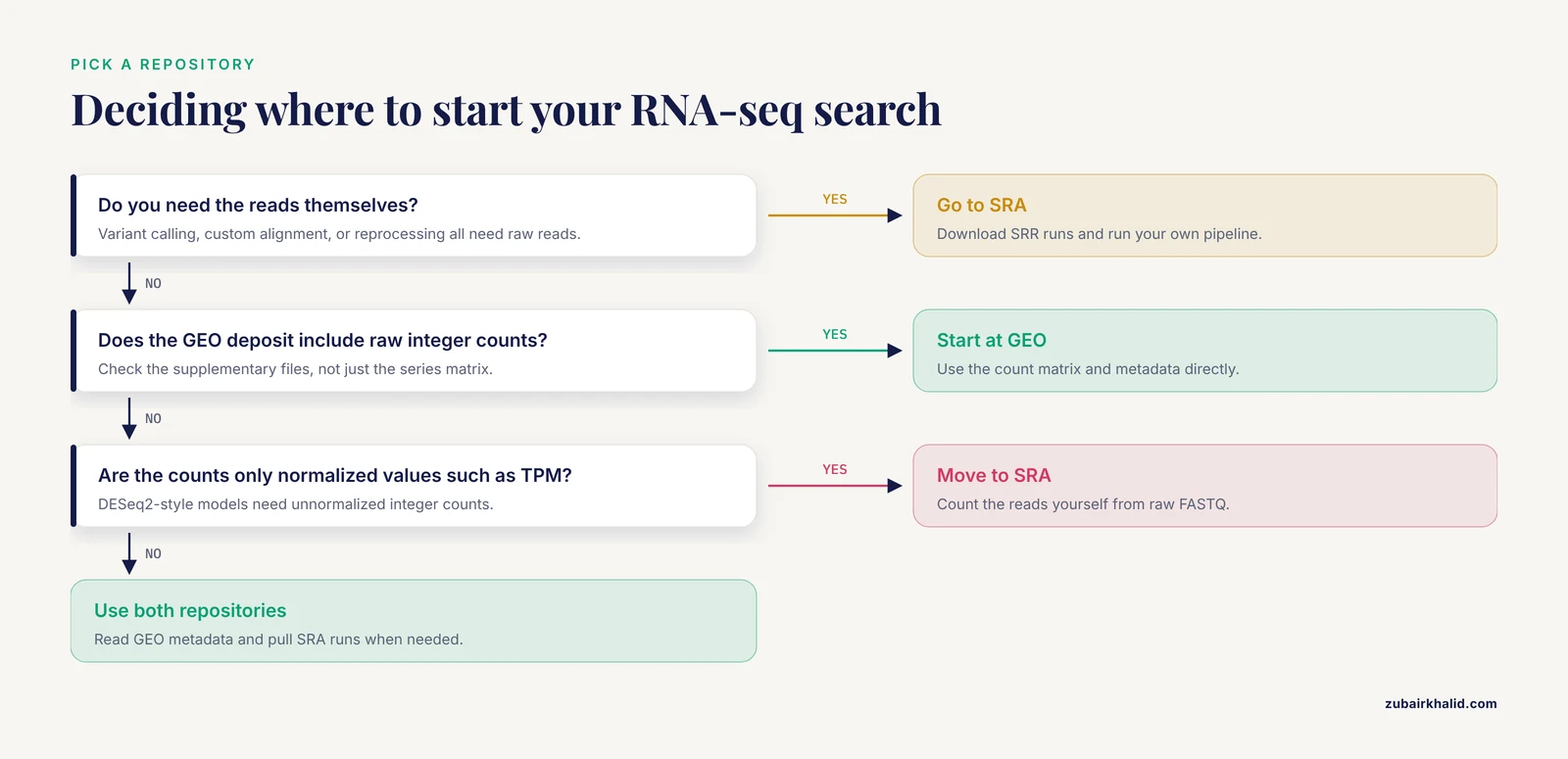
Four criteria settle most choices: your analysis goal, your compute budget, the genome build and annotation you need, and how sensitive your question is to processing choices.
| Your goal | Start at | Move to SRA when |
|---|---|---|
| Reanalyze a published comparison | GEO counts | Counts are absent or provided only as normalized values |
| Meta-analysis across studies | GEO metadata and counts | Batch effects demand uniform reprocessing of raw reads |
| Variant calling or allele-specific analysis | SRA | Always, because count tables discard sequence variation |
| Single-cell reprocessing | GEO for matrices | You need Cell Ranger runs from FASTQ |
| Non-model organism analysis | GEO counts if present | The genome build or annotation version matters |
| QC audit of a published paper | SRA | You must verify the reads support the claims |
Compute is the practical divider. A GEO supplementary download takes seconds and runs on a laptop. SRA downloads take hours, consume disk, and demand an alignment-capable machine or cloud resources. Teaching protocols now run the heavy steps on free cloud platforms such as Google Colab precisely to lower that barrier [12].
Genome build is the scientific divider. Counts are frozen to whatever reference and annotation the submitter used. If your question depends on current gene models or a current assembly, as resources like Xenbase maintain for their communities, raw reads from SRA are the only safe substrate [10].
Metadata depth differs in kind, not just degree. GEO excels at experimental design, SRA excels at per-run technical detail such as instrument and library strategy. A careful project reads both.
Finally, know the middle ground. GREIN provides uniformly processed GEO datasets when you want more consistency than raw supplementary files but less effort than full reprocessing [5]. GEfetch2R handles fetching from both repositories inside R [8].
Worked Scenarios
Scenario 1: Build a Biomarker Classifier From Published Counts
Your goal is to train a classifier on a published disease contrast without sequencing anything. Search GEO for the disease and RNA-seq, pick a series with raw counts in the supplementary files, confirm sample sizes and design on the series page, download the count matrix and metadata, and proceed in R. The autism biomarker study followed essentially this path, drawing its cohorts from GEO and feeding processed values into random forest and XGBoost models with five-fold cross-validation [6]. Check early that the matrix holds raw integer counts rather than normalized values, because count-based models expect raw counts.
Scenario 2: Pool Several Studies Into One Meta-Analysis
Your goal is to find genes consistent across independent cohorts. Collect several GEO series for the same disease, harmonize gene identifiers, analyze each series separately, then combine results. The pancreatic cancer meta-analysis pooled seven GEO datasets with a new local cohort and found five cell cycle regulator genes, including CDC20 and PLK1, concordant across all of them [7]. Where cohorts used different library kits or pipelines, consider pulling raw reads from SRA and reprocessing everything identically, because library generation and analysis choices can manufacture signals that fail to validate [11].
Scenario 3: Detect Variants in Candidate Genes From Public RNA-Seq
Your goal is to genotype expressed genes when genome sequencing data is scarce. Identify a BioProject with RNA-seq from the relevant tissue, list its SRR runs in the Run Selector, download with prefetch and fasterq-dump, align to the reference genome, and call variants in expressed regions. The opioid use disorder study did this with ventral midbrain RNA-seq under PRJNA492904, screening candidate genes for variants that could alter protein function [3].
Scenario 4: Reprocess a Single-Cell Dataset Under Your Own Settings
Your goal is to apply current tools and references to a published single-cell study. Take the count matrix from GEO for a first look, then pull raw FASTQ from the linked BioProject for a full reprocessing pass. The salivary gland single-nucleus study pairs GEO accession GSE176155 with BioProject PRJNA735197, and its secondary analysis ran raw FASTQ through Cell Ranger v6.0.1 aligned to GRCh38 before clustering and annotation in Seurat [2]. GEfetch2R automates the fetching side for both raw and processed single-cell data [8].
Scenario 5: Analyze RNA-Seq for a Non-Model Organism
Your goal is to extract biology from an organism with sparse annotation. If a GEO series provides counts, start there and spend your effort on annotation quality instead, building custom annotation packages from NCBI data for enrichment analysis, as demonstrated for Mycobacterium tuberculosis with dataset GSE292409 [9]. If you must generate counts yourself, run a raw pipeline from SRA, as the PipeSeq developers did for Chlamydomonas reinhardtii, chaining SRA Toolkit, HISAT2, StringTie, featureCounts, and DESeq2 on raw SRA datasets [13].
How to Download Data From GEO and SRA
Most of learning how to use NCBI efficiently comes down to reading accession pages carefully and following the links between databases. The two workflows below cover the common cases.
Downloading From GEO
- Search at www.ncbi.nlm.nih.gov/geo by accession or keywords, and filter to expression profiling by high throughput sequencing to restrict to RNA-seq.
- On the series page, use the Supplementary file download link, or browse the FTP directory directly.
- The FTP pattern nests series by prefix. For GSE65117 the directory is https://ftp.ncbi.nlm.nih.gov/geo/series/GSE65nnn/GSE65117/suppl/, where the GSE65nnn segment takes the first three digits of your accession followed by nnn. File names vary by submitter and commonly include raw counts, normalized tables, and metadata sheets.
- In R, the GEOquery package pulls series metadata and processed tables directly:
library(GEOquery)
gse <- getGEO("GSE65117")
The series matrix file carries sample metadata. For RNA-seq, the expression values usually sit in the supplementary files rather than the series matrix itself, so check the supplementary directory for the count matrix.
Downloading From SRA
- From the GEO series page or the BioProject page, open the SRA link, then open the Run Selector to list every SRR run with per-run metadata such as instrument, layout, and read counts.
- Install sra-tools and fetch the runs you need:
conda install -c bioconda sra-tools
prefetch SRRXXXXXXX
fasterq-dump SRRXXXXXXX --split-files --threads 8
pigz *.fastq
prefetch downloads the compressed SRA file into a local cache. fasterq-dump converts it to FASTQ, and, split-files separates paired-end data into two files, one per mate. pigz compresses the output in parallel. The older fastq-dump still works for single runs but is slower on large jobs. For a multi-run project, write a loop over a list of run accessions and plan storage before you start, since converted FASTQ files run to multiple gigabytes per sample.
Tools That Bridge Both Repositories
Several resources reduce the friction of working across GEO and SRA. GREIN provides uniform processing and interactive analysis for GEO RNA-seq datasets [5]. GEfetch2R fetches raw data from SRA and ENA and count matrices from GEO into a single R workflow [8]. AOE searches across GEO, ArrayExpress, and SRA-derived RNA-seq collections [4]. RNA-Seq Viewer visualizes genome-wide expression data drawn from both SRA and GEO [14]. Specialized databases build on the same pair of archives, as DASHR 2.0 does for human small non-coding RNAs by integrating more than 800 curated experiments from ENCODE and GEO/SRA across two genome builds [15].
Common Mistakes and Limitations
- Assuming every GEO series has raw reads behind it, and every SRA study has a GEO mirror. Verify the cross-links before you plan an analysis, and remember that some RNA-seq data exists only in SRA [4].
- Feeding normalized values to tools that expect raw counts. DESeq2-style differential expression models require unnormalized integer counts. If the matrix header says TPM or FPKM, locate the raw count file in the same deposit or go to SRA and count the reads yourself.
- Ignoring the library protocol. A QuantSeq 3' mRNA-Seq kit produces strand-specific reads concentrated at transcript 3' ends, as in a maize mycorrhiza dataset built with the Lexogen kit [16]. Counting behavior and interpretation differ from full-length polyA protocols, so read the series description before assuming standard gene-body coverage.
- Confusing accession namespaces. GSE and GSM belong to GEO, SRP, SRX, and SRR belong to SRA, and PRJNA and SAMN belong to BioProject and BioSample. Published articles sometimes blur these labels, describing a PRJNA accession as a GEO accession [3], so always verify by prefix before querying.
- Underestimating raw data logistics. Converted FASTQ files occupy multiple gigabytes per sample, and a forty-run project can exceed a laptop's disk. Prefetch selectively, compress immediately, or push heavy steps to cloud infrastructure, as current teaching protocols do with Google Colab [12].
- Treating processed values from different studies as directly comparable. Pipelines, genome builds, and library kits differ across deposits, and those differences can generate signals stronger than the underlying biology, as the allele-specific expression meta-analysis demonstrated [11].
- Ignoring software versions during reprocessing. One single-cell reanalysis pinned Cell Ranger v6.0.1 and Seurat v4.0.5 [2], and different versions yield different counts from the same FASTQ files. Record every version for reproducibility.
- Skipping the metadata hunt. Sample-level annotations live in the GEO series matrix, run-level technical details live in the SRA Run Selector, and a correct batch-aware model usually needs both.
Every dataset and question differs, and high-stakes analyses deserve review by an experienced bioinformatician or statistician before publication or clinical use.
Frequently Asked Questions
Should you use GEO or SRA for RNA-seq data?
Use GEO when you want processed count matrices, sample metadata, and study design, and use SRA when you need the raw reads for your own pipeline. Most projects touch both, starting at GEO and pulling runs from SRA only when the analysis demands raw data.
Can I download raw FASTQ files directly from GEO?
Usually no. GEO hosts processed files such as count matrices, and raw reads normally live in SRA through a linked BioProject, so follow the SRA link on the GEO series page to reach the FASTQ data.
Why do some GEO entries have no linked raw reads?
Older submissions and some non-standard deposits predate strict linking or never uploaded reads to SRA. Search SRA or a cross-repository index such as AOE directly, because some RNA-seq data exists in SRA with no GEO entry at all.
Do I need raw reads from SRA for differential expression analysis?
Not usually. If the GEO deposit includes raw gene-level counts and clear metadata, you can run DESeq2 or edgeR directly, and platforms like GREIN supply uniformly processed GEO datasets. Reach for SRA when counts are missing, provided only as normalized values, or generated in ways you cannot trust for your question.
What do GSE, GSM, SRR, and PRJNA accessions mean?
GSE identifies a GEO series, GSM identifies a GEO sample, SRR identifies an SRA run of reads, and PRJNA identifies a BioProject study umbrella. Matching these prefixes tells you which database to query and prevents wasted searches in the wrong repository.
How do I find RNA-seq studies that are not indexed in GEO?
Search SRA directly through its web interface or the Run Selector, or use a cross-repository index such as AOE, which collects RNA-seq data from SRA that never reached GEO or ArrayExpress.
Sources
- Gene expression profiling by high throughput sequencing to determine signatures for the bovine receptive uterus at early gestation.
- Expression analysis of epithelial membrane protein 1 (EMP1) gene in kidney stone patients.
- Identification of variants from gene expression data of opioid-addicted patients.
- All of gene expression (AOE): An integrated index for public gene expression databases.
- GREIN: An Interactive Web Platform for Re-analyzing GEO RNA-seq Data.
- Identification of Potential Biomarkers in ASD Integrating RNA Seq Data and Machine Learning Approaches.
- Dysregulated expression of cell cycle regulators CDC20, PLK1, BUB1, CDC45, CDCA5 in pancreatic ductal adenocarcinoma.
- GEfetch2R: fetching single-cell/bulk RNA-seq data from public repositories to R and benchmarking the subsequent format conversion tools.
- Enhanced RNA-Seq Expression Profiling and Functional Enrichment in Non-model Organisms Using Custom Annotations.
- Xenbase: deep integration of GEO & SRA RNA-seq and ChIP-seq data in a model organism database.
- Reassessment of weak parent-of-origin expression bias shows it rarely exists outside of known imprinted regions.
- Streamline Protocol for Bulk-RNA Sequencing: From Data Extraction to Expression Analysis.
- Development and validation of the PipeSeq program for RNA-seq data analysis in the Chlamydomonas reinhardtii as a model.
- Viewing RNA-seq data on the entire human genome.
- DASHR 2.0: integrated database of human small non-coding RNA genes and mature products.
- Illumina RNA-seq data of Genotype-specific responses of maize plants to Funneliformis mosseae.