How to Estimate Cloud Storage and Compute Costs for Genomics

By Dr. Zubair Khalid, DVM, MS, PhD · 2026-11-11

By the end of this article you will be able to produce a defensible cost estimate for a genomics analysis run in the cloud, before you spend a dollar on it. You will build a small estimator script, benchmark a real workflow on a subset of your data, extrapolate to full scale, and sanity-check your numbers against published cloud genomics results. You will also learn where estimates go wrong, because underestimating storage in particular is a failure mode with real precedent.

To follow along you need three things on hand. First, a spreadsheet or a Python 3 installation for the arithmetic. Second, the pricing pages or cost calculator for your provider, such as the AWS Pricing Calculator for aws genomics workloads, because list prices change and you should never copy a rate out of a tutorial, including this one. Third, a rough inventory of your data: how many samples, how many gigabytes of raw reads per sample, which tools you plan to run, and how long each tool takes per sample on hardware you have access to. If you do not know runtimes yet, the walkthrough below shows how to get them with a small benchmark before committing to full-scale execution.

Why Estimating Before You Run Matters

Cloud computing removed the capital cost of owning a compute cluster, but it replaced that problem with a different one: uncertainty about what a given analysis will actually cost. This concern has a name in the literature, the "bioinformatics bottleneck", and it refers to the uncertainty researchers face about the cost and infrastructure needed to meet sequencing analysis demands [1].

The good news is that genomics cloud costs are unusually estimable, for two reasons. First, most workflows are embarrassingly parallel across samples, so cost scales nearly linearly with sample count once you know the per-sample cost. Second, a decade of published cloud bioinformatics case studies gives you anchors to check your arithmetic against. An early and still instructive example is the Roundup comparative genomics project, which computed orthologous relationships for 245,323 genome-to-genome comparisons across 902 genomes on Amazon's Elastic Compute Cloud in just over 200 hours of computation at a cost of $8,000, using a model that predicted cloud runtime from the size and complexity of the genomes being compared in order to schedule jobs optimally [2]. A more recent example processed more than 126,000 CT volumes for AI segmentation using over 21,000 virtual machines across Terra and Seven Bridges Cancer Genomics Cloud platforms, finishing in under 9 hours instead of the estimated 522 days on a single workstation, at a total cost of $1,011.05 [3]. Both projects estimated before they ran, then benchmarked to confirm.

Skipping the estimate is where projects get into trouble, and the failure mode is usually storage rather than compute. When Queensland Genomics built a local Australian cache of seventeen bacterial species from NCBI's Sequence Read Archive, the initial storage estimation did not keep up with the exponential growth of reads being uploaded to SRA, a lesson in why storage projections need growth assumptions built in from day one [4].

The Anatomy of a Genomics Cloud Bill

Before you can calculate anything, you need to know what a genomics cloud bill actually consists of. Five components account for essentially everything.

Compute

Compute is the cost of virtual machine (VM) time, measured in instance-hours. A virtual machine is a rented slice of a physical server, sold in types that bundle a certain number of virtual CPUs (vCPUs), memory, and sometimes GPUs. Compute is usually the largest line item for reprocessing runs and the most controllable one, because you choose the instance type. The Trans-Proteomic Pipeline project compared the relative performance and costs of various EC2 instance types for shotgun proteomics and found the choice materially changed both runtime and cost, which is the general rule in cloud bioinformatics [5]. For GPU workloads the choice matters even more. The GoToCloud cryo-EM platform ran detailed economic analyses to identify which GPU instance types, such as NVIDIA T4 versus A10G, balanced processing speed against expense, and found a "2.0 Å wall" in cost-performance for structure refinement beyond a certain resolution target [6].

Storage

Storage is charged in GB-months, meaning you pay a monthly rate multiplied by the number of gigabytes you hold and the number of months you hold them. Genomics storage has a distinctive shape: raw data is large and permanent, while intermediate files (aligned BAMs, indexes, temp files) can be several times the size of the raw data but should be deleted after the pipeline finishes. Whole-genome bisulfite sequencing pipelines, for example, are designed to handle 100 GB or more of raw data per sample, which gives you a sense of scale for epigenomic workloads [7].

Data transfer and egress

Egress is data leaving the provider's network, such as downloading results to your lab. Inbound transfer to the cloud is typically free, outbound transfer is charged per GB, and transfer between regions or between certain services can also be charged. For most genomics projects egress is small relative to compute, but for projects that repeatedly move large result sets off the cloud it can become significant.

Requests and small-file overhead

Object storage providers charge small per-request fees for reads and writes. This is negligible for a few hundred BAM files and meaningful for pipelines that write millions of small shard files. File count, not just file size, belongs in your estimate.

Managed platform and orchestration overhead

If you run on a managed genomics platform rather than raw VMs, the platform adds its own charges on top of the underlying infrastructure. The National Cancer Institute-funded Cancer Genomics Cloud, for example, supports cloud-hosted collaborative projects with compute hardware from providers such as Amazon Web Services and Google Cloud Platform, and such platforms bundle execution, data management, and collaboration features into their pricing [8].

The table below summarizes the components and the formula terms they map to.

Cost component	Formula term	Main drivers	How to measure it
Compute	Σ (instance-hours × rate)	Number of tasks, runtime per task, instance size	Benchmark a few samples
Storage	Σ (GB-months × rate)	Raw data volume, intermediates, retention time	File inventory with `du` or storage metrics
Egress	GB out × rate	Downloads to your lab, cross-region copies	Data inventory of outputs
Requests	Count × rate	Number of small files written	File counts from a test run
Platform overhead	Platform fee × usage	Managed platform pricing model	Platform documentation
Waste	Idle instances, orphaned disks	Cleanup discipline	Billing report after a test run

How to Calculate Cloud Storage and Compute Costs for Genomics: The Formula

The estimate cloud storage compute genomics formula that covers nearly every scenario is:

Total cost = Compute + Storage + Egress + Requests + Platform fees + Contingency

Compute  = (total vCPU-hours or instance-hours) × (price per hour)
Storage  = (total GB held) × (price per GB-month) × (months held)
Egress   = (GB transferred out) × (price per GB)
Requests = (number of API operations) × (price per operation)
Contingency = 20% to 50% of the subtotal, depending on estimate maturity

The hard part is not the arithmetic, it is estimating the two quantities you control least: total instance-hours and total GB held. Break each down further.

For compute, decompose instance-hours into parallelism:

Total instance-hours = (tasks per sample)
                     × (average runtime per task in hours)
                     × (instances running in parallel)
                     × (number of samples)
                     ÷ (parallel efficiency)

Parallel efficiency accounts for the fact that the last stragglers of a batch keep instances billing while other instances sit idle. For uniform tasks efficiency approaches 1. For variable tasks, such as assembly where some genomes finish in 20 minutes and some in 6 hours, efficiency can drop to 0.6 or worse, and you pay for the idle tail.

For storage, decompose by data class:

Total GB = raw GB + intermediate GB + reference and index GB + result GB
GB-months = Σ over each class of (GB × months retained)

A useful heuristic for pipeline storage is to price intermediates at 3 to 5 times raw data volume during the run window, then drop them to near zero after the run. What you must not do is assume storage stays flat. The SRA cache project in Australia watched its data holdings grow exponentially as sequencing output worldwide increased, which is why any multi-year storage estimate needs an annual growth multiplier, commonly 1.5x to 2x per year for actively growing sequencing collections [4].

The Roundup project demonstrated the value of the runtime term specifically. Rather than guessing, its authors created a model to estimate cloud runtime based on the size and complexity of the genomes being compared, and used that model to determine the optimal order of job submission, maximizing use of the cloud while minimizing cost [2]. Runtime prediction is the highest-leverage variable in the whole formula, so the walkthrough below invests most of its effort there.

Step-by-Step Walkthrough: Building Your Estimate

The following procedure takes you from nothing to a defensible number. Each step includes commands or code and what the output should look like.

Step 1: Inventory your data

Measure, do not guess, the size of your input data. If the data is already in cloud object storage, use the provider's listing tools. On AWS:

# Sum the size of all objects under a prefix
aws s3 ls s3://my-lab-bucket/fastq/ --recursive --summarize \
  | grep "Total Size"

# Count the files, which drives request costs
aws s3 ls s3://my-lab-bucket/fastq/ --recursive | wc -l

Expected output looks like this:

2026-01-14 09:22:31  31250000000   2024-06-12 00:00:00 sample_001_R1.fastq.gz
...
Total Objects:        1500
Total Size:           15000000000000

That is 1,500 objects totaling 15,000,000,000,000 bytes, which is 15,000 GB or 15 TB (using the decimal convention object storage bills in). If your data is local, du -sb /data/fastq/ gives the byte-accurate total and find /data/fastq/ -type f | wc -l gives the file count.

Step 2: Determine per-task runtime with a pilot

Pick one representative sample and run the heaviest step of your pipeline on it, on the instance type you intend to use. Track wall-clock time. If you use Nextflow or Snakemake, the run report already contains per-process runtimes:

nextflow run main.nf -profile test -with-report pilot_report.html

The generated report lists each process with its duration. For a single manual step, time it directly:

time bwa mem -t 8 reference.fa sample_001_R1.fq sample_001_R2.fq > sample_001.sam

Expected output:

real  47m12.5s
user  289m3.1s
sys   4m51.2s

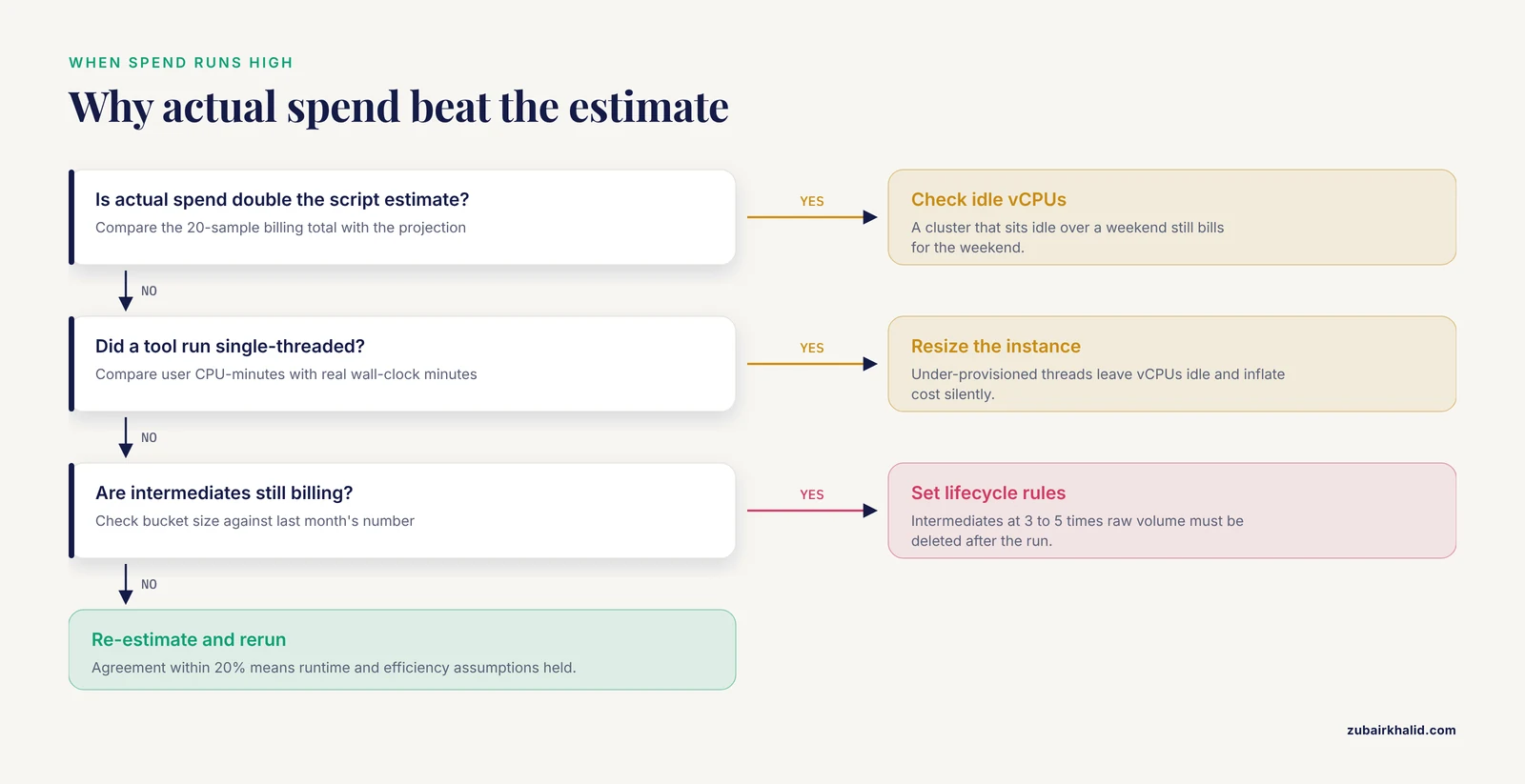
The real value is what you bill for. The gap between user and real here (289 CPU-minutes versus 47 wall-clock minutes) tells you the job is using about 6 cores in parallel, which confirms the -t 8 flag is roughly being used and helps you size instances correctly. Under-provisioned threads that leave vCPUs idle are a common source of silent cost inflation.

Step 3: Write the estimator script

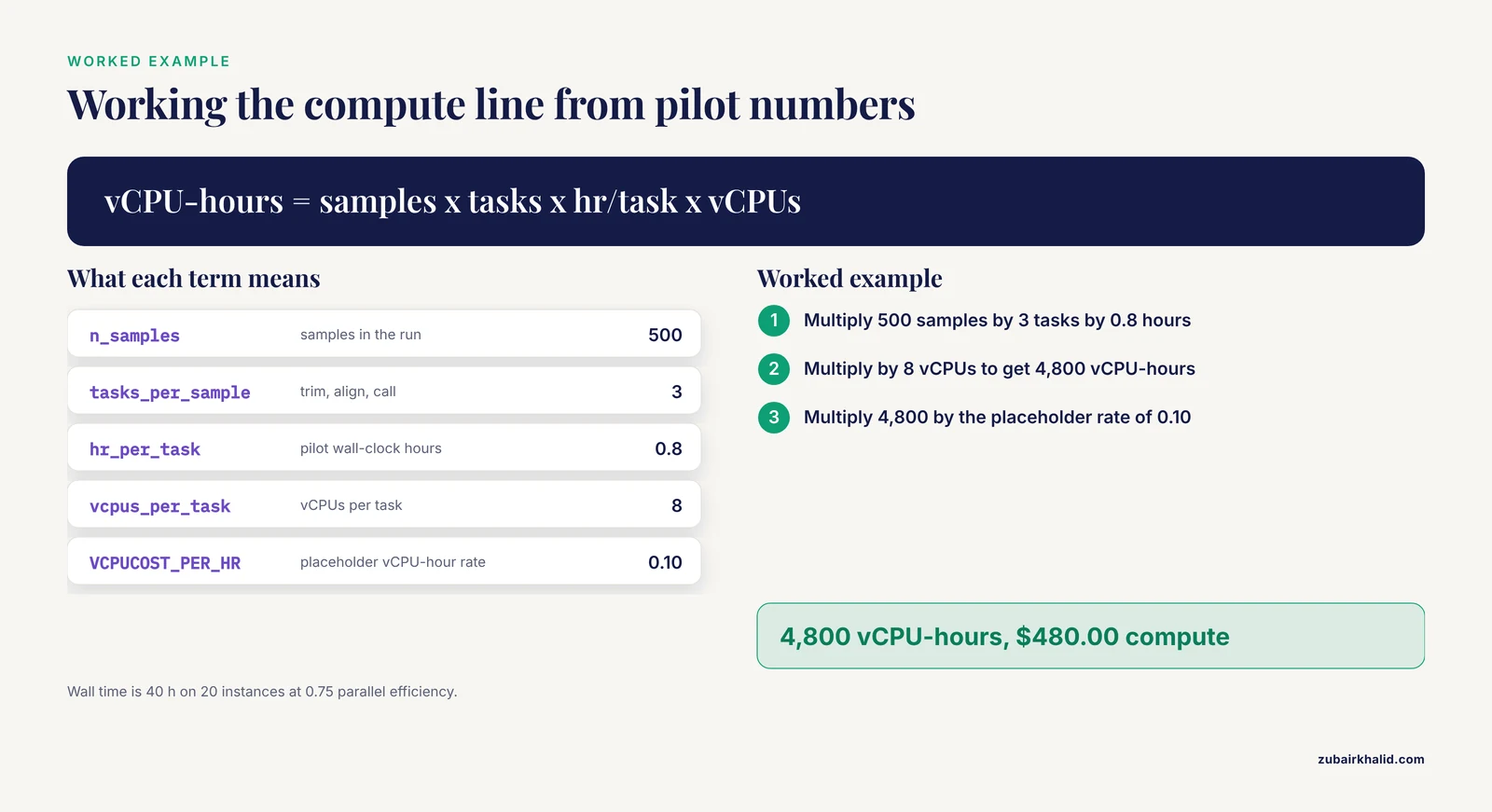
Calculation of total vCPU-hours and compute cost from 500 samples, 3 tasks, 0.8 hours per task and 8 vCPUs, giving 4,800 vCPU-hours and $480.00.

Put the measured numbers into a script so the estimate is reproducible and auditable. All rates below are illustrative placeholders. Replace each one with the current rate from your provider's pricing page before using the output for anything real.

# cloud_cost_estimator.py
# All rates are ILLUSTRATIVE PLACEHOLDERS. Substitute current
# published prices from your provider before acting on the output.

# Rates (placeholders)
VCPUCOST_PER_HR   = 0.10   # dollars per vCPU-hour
STORAGE_PER_GB_MO = 0.022  # dollars per GB-month, standard tier
EGRESS_PER_GB     = 0.09   # dollars per GB out
REQUESTS_PER_10K  = 0.05   # dollars per 10,000 object operations

# Workload inputs (from your inventory and pilot)
n_samples        = 500
tasks_per_sample = 3          # trim, align, call
hr_per_task      = 0.8        # from pilot benchmark
vcpus_per_task   = 8
parallel_instances = 20
parallel_efficiency = 0.75    # 0.75 means 25% waste in the tail

raw_gb_per_sample = 30        # from Step 1
intermediate_multiplier = 4   # intermediates during the run
run_window_months = 0.25      # one week of run time
retain_years      = 3         # raw + results retained

# Compute
total_vcpu_hours = (n_samples * tasks_per_sample * hr_per_task
                    * vcpus_per_task)
wall_hours = (n_samples * tasks_per_sample * hr_per_task
              / parallel_instances / parallel_efficiency)
compute_cost = total_vcpu_hours * VCPUCOST_PER_HR

# Storage
raw_gb      = n_samples * raw_gb_per_sample
mid_gb      = raw_gb * intermediate_multiplier
storage_cost = (raw_gb + mid_gb) * STORAGE_PER_GB_MO * run_window_months \
             + (raw_gb) * STORAGE_PER_GB_MO * retain_years * 12

# Egress and requests
result_gb   = raw_gb * 0.3
egress_cost = result_gb * EGRESS_PER_GB
n_files     = n_samples * 12
request_cost = (n_files / 10_000) * REQUESTS_PER_10K

subtotal = compute_cost + storage_cost + egress_cost + request_cost
contingency = 0.4 * subtotal

print(f"Compute wall time   : {wall_hours:,.0f} h "
      f"({wall_hours/24:.1f} days)")
print(f"Compute vCPU-hours  : {total_vcpu_hours:,.0f}")
print(f"Compute cost        : ${compute_cost:,.2f}")
print(f"Storage cost        : ${storage_cost:,.2f}")
print(f"Egress cost         : ${egress_cost:,.2f}")
print(f"Request cost        : ${request_cost:,.2f}")
print(f"Subtotal            : ${subtotal:,.2f}")
print(f"Total with 40% buffer: ${subtotal + contingency:,.2f}")

Expected output:

Compute wall time   : 40 h (1.7 days)
Compute vCPU-hours  : 4,800
Compute cost        : $480.00
Storage cost        : $1,417.86
Egress cost         : $405.00
Request cost        : $0.03
Subtotal            : $2,302.89
Total with 40% buffer: $3,224.05

Notice two things about this output. Storage dominates, not compute, because three years of retention at 15 TB dwarfs a 40-hour compute burst. And the parallelism math shows the full batch finishes in under two days on 20 instances, which is the number that actually decides whether the cloud approach beats your local queue.

Step 4: Sanity-check against published anchors

Run the same arithmetic backward on published results to calibrate your instincts. These are the anchors worth memorizing.

The Roundup orthology computation cost $8,000 for roughly 200 hours of cloud computation, which is about $40 per hour of cluster time, and about 3.2 cents per genome-to-genome comparison across 245,323 comparisons [2]. If your per-unit cost lands within an order of magnitude of comparable published work, your estimate is probably structurally sound. The medical imaging curation study cited earlier spent $1,011.05 across more than 21,000 VMs, which is under 5 cents per VM, achievable because each task was short and the platform batched aggressively [3]. For cryo-EM, laboratories can determine high-resolution single-particle structures on the cloud for $50 to $1,500 per structure depending on data volume and refinement depth, a useful range for structural genomics budgeting [9]. For microbial genomics, benchmark costs and runtimes differ considerably by application: 16S rRNA analyses completed on a single-CPU desktop in under three hours, while whole-genome shotgun assembly, annotation, and metagenomics carried far heavier requirements, so per-application-type costing is essential rather than per-basepair costing [1].

Step 5: Refine with a scaled benchmark

Decision path for a run that costs more than estimated, testing idle instances, single-threaded tools and intermediates before re-estimating.

A pilot on 1 sample proves the pipeline runs. A scaled benchmark on 20 samples proves the estimate scales. Run 20 samples, record actual cost from your billing console, and compare:

# After the scaled run, pull actual spend for the tag you assigned
aws ce get-cost-and-usage \
  --time-period Start=2026-11-01,End=2026-11-15 \
  --granularity DAILY \
  --metrics UnblendedCost \
  --filter '{"Tags":{"Key":"project","Values":["pilot20"]}}'

Expected output is a JSON block with daily cost entries summing to, for example, $92.40. If 20 samples cost $92.40, the measured per-sample compute cost is $4.62, and 500 samples project to $2,310 plus storage and egress, which you can compare directly with the script estimate of $480. Agreement within 20% means your runtime and parallel-efficiency assumptions were reasonable. If actual spend is double the estimate, suspect idle vCPUs, a tool that silently runs single-threaded, or storage accumulation from intermediates that never got deleted.

Choosing Instance Types and Parallelization Wisely

The instance type decision is where the same analysis can double or halve in cost. Published cloud genomics work gives consistent guidance on how to approach it.

First, benchmark instance types against each other rather than trusting intuition. The Trans-Proteomic Pipeline team compared EC2 instance types explicitly for proteomics search workloads and published the relative performance and cost tradeoffs [5]. The GoToCloud cryo-EM platform went further and identified specific GPU types, NVIDIA T4 versus A10G, as the cost-performance sweet spot for their refinement workloads, validating the choice with benchmarking on real datasets [6]. The pattern in both cases is the same: measure throughput per dollar on your actual workload, not on a generic benchmark, and pick the instance class with the best jobs-per-dollar.

Second, size clusters to the workload. The cryo-EM cloud environment from Cianfrocco and Leschziner supported clusters scaling from 16 to more than 480 CPUs and showed that this off-the-shelf approach delivered results in timeframes comparable to local clusters, meaning you should scale the cluster to the deadline you have, then let cost follow [9]. If the run can take a week on cheap capacity instead of a day on premium capacity, the week is usually far cheaper.

Third, be aware that more parallelism is not automatically better on every axis. The carbon footprint analysis of bioinformatics found that using faster processors or greater parallelization reduces running time but can lead to a greater carbon footprint, and that memory over-allocation is a substantial hidden contributor to emissions [10]. The same over-provisioning that inflates your bill inflates your environmental cost, which makes careful runtime measurement doubly worthwhile.

Storage Estimation in Detail

Storage deserves its own section because it is the component most often underestimated and the one that persists after the compute is long gone. Three practices fix most storage estimation problems.

First, inventory every data class and assign each a lifetime. Raw FASTQ files, aligned BAMs plus their indexes, variant call files, reference genomes and their indices, and per-task temp directories all have different sizes and different retention needs. The methylation preprocessing pipelines designed for cloud execution handle 100 GB or more of raw data per sample for whole-genome bisulfite sequencing, which illustrates how quickly per-sample storage scales even before intermediates [7]. Write the lifetime into the estimate, as the script in Step 3 does, and hold yourself to it.

Second, build growth into multi-year projections. The Australian SRA cache experience is the canonical warning: a storage plan calibrated to current data volumes could not keep pace with the exponential growth in deposited sequencing reads [4]. For any dataset you expect to keep adding to, multiply year-one storage by a growth factor and price the out-years explicitly.

Third, check the result. Object storage consoles report bucket size and growth over time, and a monthly review against your projection catches drift while it is still cheap to fix:

aws s3 ls s3://my-lab-bucket/ --recursive --summarize | grep "Total Size"
# Compare with last month's number and verify the delta matches
# what your pipeline actually produced

Platforms and Orchestration Choices

Raw infrastructure is not the only option, and the platform you choose changes the cost structure you estimate against. Managed science platforms such as Terra (FireCloud) and the Seven Bridges Cancer Genomics Cloud let you run workflows like TotalSegmentator at massive scale, as the 21,000-VM imaging study demonstrated, and handle batching and cleanup that you would otherwise script yourself [3]. The Cancer Genomics Cloud similarly packages AWS and Google Cloud hardware behind collaborative project management [8]. The trade is convenience and reproducibility features for an additional pricing layer, which you should obtain from the platform's own documentation and add as the "Platform fees" term in the formula.

If you orchestrate yourself, workflow engines keep costs honest because they clean up and they record runtimes. GenePy, a gene-burden scoring workflow, was deployed as a containerized Nextflow pipeline integrated within the Genomics England Research Environment via the Lifebit CloudOS platform, with modular processes designed for high-throughput execution on cloud-native infrastructure [11]. Federated designs add another pattern: Fedflow orchestrates federated learning tasks across distributed VMs within the FeatureCloud platform, embedded in Snakemake workflows for reproducibility, which matters for cost because federated runs bill across multiple sites simultaneously [12]. Newer cloud-native frameworks such as Bio-OS align with GA4GH standards including the Workflow Execution Service, Task Execution Service, Data Repository Service, and Tool Registry Service, and standard interfaces make it easier to move a workload to cheaper infrastructure later because the workflow description does not change [13].

Whatever you choose, tag every resource with a project code and review the billing report after every pilot. The billing report is the ground truth that turns a first-run estimate into a second-run prediction.

Sustainability and the Carbon Dimension

Cost and carbon track each other closely in cloud bioinformatics, and the same levers reduce both. Using the Green Algorithms calculator, researchers estimated the carbon footprint of common bioinformatic analyses in kilograms of CO2 equivalent and found that software choices matter enormously: upgrading BOLT-LMM from v1 to v2.3 reduced the carbon footprint of biobank-scale GWAS by 73%, and moving computation from an average data center to a more efficient one reduced it by approximately 34% [10]. Since cloud providers publish data center efficiency characteristics, region selection is both a cost and a sustainability decision. Include carbon in your estimate when your institution reports emissions, using the same runtime and instance inputs you already computed for the dollar estimate.

Common Mistakes and Limitations

Every point below is a real failure mode seen in practice.

Guessing runtimes instead of benchmarking. Runtime is the highest-leverage variable in the formula, and a 2x error multiplies through the entire compute line. Always run the pilot and the 20-sample scaled benchmark before trusting an extrapolation.
Estimating storage at raw-data size only. Intermediates commonly reach 3 to 5 times raw volume during the run, and forgotten intermediates billing for months are the classic silent cost leak. Assign lifetimes and enforce them with lifecycle rules.
Treating storage as static in multi-year plans. The SRA cache project watched initial storage estimates fail against exponential data growth, so out-year storage needs a growth multiplier [4].
Ignoring parallel efficiency. A batch of 1,000 uneven assembly jobs keeps a full fleet billing through the long tail. Use the efficiency factor in the formula, and schedule long jobs first as the Roundup authors did to maximize utilization [2].
Picking instance types by intuition. Published cloud genomics studies consistently found instance selection changes cost materially, and benchmarked explicitly before choosing [5][6].
Confusing wall time with billed time. A cluster that finishes in 2 days but sits idle over a weekend bills for the weekend. Terminate clusters explicitly and automate cleanup.
Forgetting requests and small files. Pipelines that shard heavily can generate request charges that rival storage charges.
Treating the estimate as a contract. A first-pass estimate with a 40% contingency is a planning number, not a guarantee. The scaled benchmark is what turns it into a forecast.
Over-provisioning memory. Memory over-allocation is a substantial contributor to both cost and carbon footprint, so right-size after the pilot rather than defaulting to the largest instance [10].
A final limitation: estimates are only as good as the workload definition behind them. If the analysis changes mid-project, re-estimate.

Frequently Asked Questions

How accurate is a first-pass cloud cost estimate for genomics?

Expect a first-pass estimate built from a single-sample pilot to be within roughly 20 to 50% of actual spend, which is why you carry a contingency term. A 20-sample scaled benchmark typically tightens this to within about 20%. The published anchors from cloud genomics case studies give you a realism check on the order of magnitude before you spend anything [2][3].

Do I pay to move data into the cloud?

Inbound transfer to cloud object storage is typically free, while outbound transfer, called egress, is charged per GB. The egress term matters most for projects that repeatedly download large results. Check your provider's current transfer pricing rather than assuming any rate.

Can spot or preemptible instances reduce the bill?

Yes, providers sell spare capacity at large discounts, and batch genomics workloads tolerate interruptions well when the workflow engine resumes from checkpoints. Test your pipeline's restart behavior on a small batch before committing a large run to discounted capacity, and confirm current discount rates on the provider's pricing page.

How much storage does one whole genome sample take?

It depends on the assay and coverage, so measure your own data with du or storage metrics rather than borrowing a number. For scale, whole-genome bisulfite sequencing pipelines are designed around 100 GB or more of raw data per sample [7]. Remember to budget intermediates during the run at several times raw volume.

Should I use a managed platform like Terra or a raw cloud account?

A managed platform adds a pricing layer but handles batching, cleanup, collaboration, and reproducibility infrastructure, and large studies have run successfully on Terra and Seven Bridges platforms [3][8]. If your team lacks dedicated infrastructure staff, the platform fee is often cheaper than the engineering time to replicate those features.

How do GPU workloads change the estimate?

GPU instances cost more per hour, so the runtime reduction has to be large enough to win on cost per completed job. Benchmark GPU types against your actual workload as the GoToCloud project did when comparing NVIDIA T4 and A10G instances for cryo-EM refinement [6]. Include GPU memory in the sizing check, because over-allocated GPU memory bills the same as over-allocated CPU memory.

What is the most common reason cloud genomics projects go over budget?

Unmanaged storage growth is the most common culprit, because compute bills end when the run ends but storage bills continue until someone deletes the data. The Australian SRA cache saw its storage estimates fail against exponential growth in deposited reads [4]. Set lifecycle policies and a monthly bucket-size review from day one.

Does cloud computing have an environmental cost I should estimate?

Yes, and it is estimable with the same inputs as the dollar estimate. The carbon footprint of bioinformatics analyses has been quantified in kgCO2e, with software version choices alone reducing footprints by as much as 73% and data center selection contributing roughly 34% reductions [10]. Compute runtime and region choice drive both your bill and your emissions.