Top 10 R Packages Every Bioinformatics Beginner Should Know
By Dr. Zubair Khalid, DVM, MS, PhD ·

The difference between doing bioinformatics in R and clicking through a web tool comes down to one sentence: in R, every decision lives in a script you can rerun, share, and defend, while a web tool hands you a result you cannot fully reconstruct. The rule of thumb for choosing packages is equally short. Install BiocManager on day one, learn DESeq2, ggplot2, and clusterProfiler for your first expression analysis, and add the rest when your data type demands them.
Beginners searching for the best essential R packages for bioinformatics usually need the same ten, because most entry-level genomics work reduces to three tasks: expression analysis, functional enrichment, and coordinate wrangling. This guide explains what each package does on its own terms, compares the ones that overlap, walks through three realistic projects, and lists the mistakes that cost newcomers the most time. Everything here runs on Windows, macOS, or Linux with the free version of R.
What R for Bioinformatics Actually Means (and Where Bioconductor Fits)
R is a programming language built for statistics. A package is an installable bundle of functions, documentation, and often example data. Two repositories matter. CRAN, the Comprehensive R Archive Network, hosts general-purpose R packages. Bioconductor hosts packages built specifically for high-throughput genomic data, and it ships shared data structures so that one package's output becomes the next package's input without conversion headaches.
Bioconductor is open source and open development, meaning the code is public and developed in the open, and published protocols have used it for years to dissect transcriptomic data [1]. That pipeline shape, transform the data, model it, then interpret it, is the template you will reuse across data types.
A minimal Bioconductor tutorial setup takes three lines:
install.packages("BiocManager")   # run once per R installation
BiocManager::install()            # set up the current Bioconductor release
BiocManager::install("DESeq2")    # install any Bioconductor package
Use install.packages() for CRAN packages and BiocManager::install() for Bioconductor packages. Both repositories are free.
One habit saves beginners more time than any other: every Bioconductor package ships a vignette, a worked example meant to be read alongside its code. Open one with browseVignettes("DESeq2") and run it line by line. A structured Bioconductor tutorial you write for yourself, one vignette at a time, beats a stack of unrunnable example code.
The 10 Essential R Packages for Bioinformatics at a Glance
| # | Package | Core job | Typical data | Repository | First function to learn |
|---|---|---|---|---|---|
| 1 | BiocManager | Installs and updates Bioconductor software | Any | CRAN | BiocManager::install() |
| 2 | DESeq2 | Differential expression from raw counts | RNA-seq count matrix | Bioconductor | DESeq() |
| 3 | edgeR | Differential expression with quasi-likelihood tests | RNA-seq count matrix | Bioconductor | DGEList() |
| 4 | limma | Linear models for arrays and counts | Microarray, RNA-seq | Bioconductor | lmFit() with eBayes() |
| 5 | ggplot2 | Layered statistical graphics | Any data frame | CRAN | ggplot() |
| 6 | pheatmap | Annotated, clustered heatmaps | Numeric matrix | CRAN | pheatmap() |
| 7 | EnhancedVolcano | Publication-ready volcano plots | Differential expression results | Bioconductor | EnhancedVolcano() |
| 8 | clusterProfiler | GO and pathway enrichment | Gene lists, ranked lists | Bioconductor | enrichGO() |
| 9 | tmod | CERNO gene set enrichment | Ranked gene lists | CRAN | tmodCERNOtest() |
| 10 | GenomicRanges | Interval arithmetic on genomes | Genomic coordinates | Bioconductor | GRanges() |
The next section explains each package, the terms it assumes you know, and the code that gets you a first result.
The Packages in Detail
1. BiocManager: The Door to Bioconductor
BiocManager is not an analysis package. It is the installer that connects R to Bioconductor and keeps every genomic package at a compatible version. Bioconductor releases twice a year, and packages within a release are tested to work together, so installing through BiocManager prevents the version mismatches that make other people's scripts fail on your machine.
BiocManager::install("edgeR")    # any Bioconductor package
BiocManager::install("tmod")     # tmod is hosted on CRAN
BiocManager::version()           # print the release you are using
Two habits to build early. Call BiocManager::install() with no arguments after a release to update your library. Print BiocManager::version() in your scripts so anyone rerunning them knows which release produced your numbers.
2. DESeq2: Differential Expression From Raw Counts
DESeq2 finds genes whose expression changes between conditions in RNA-seq data, the sequencing of a sample's RNA to count how much of each gene is transcribed. It takes raw integer counts, the tallies of reads assigned to each gene, and models them with a negative binomial distribution, a count model that absorbs the high variance typical of small experiments. Its normalization step adjusts for library size, the total number of reads per sample, so samples with more sequencing do not look more expressive.
library(DESeq2)

dds <- DESeqDataSetFromMatrix(
  countData = counts,              # genes in rows, samples in columns
  colData   = samples,             # sample metadata, one row per sample
  design    = ~ batch + condition  # include batch if it exists
)
dds <- DESeq(dds)
res <- results(dds, contrast = c("condition", "treated", "control"))

vsd <- vst(dds)                    # variance-stabilized values for QC plots
plotPCA(vsd, intgroup = "condition")
res_shrunk <- lfcShrink(dds, coef = "condition_treated_vs_control")
Check resultsNames(dds) to see the exact coefficient labels on your data. Three decisions matter. Put batch in the design formula when samples were processed on different days. Use lfcShrink to stabilize log2 fold changes for low-count genes. Report adjusted p values, never raw ones, because you are testing thousands of genes at once.
3. edgeR: The Fast, Flexible Second Opinion
edgeR does the same job as DESeq2 with a different statistical engine. It uses TMM normalization, trimmed mean of M values, which assumes most genes do not change and trims the most extreme ratios before computing scaling factors. Its quasi-likelihood framework, a testing approach with tight control over error rates, scales well to large experiments.
library(edgeR)

y <- DGEList(counts = counts, samples = samples)
y <- calcNormFactors(y)
design <- model.matrix(~ batch + condition, data = samples)
y <- estimateDisp(y, design)
fit <- glmQLFit(y, design)
qlf <- glmQLFTest(fit, coef = "conditiontreated")  # name comes from design
topTags(qlf)
Beginners ask whether DESeq2 and edgeR disagree. On well-behaved datasets they agree on most genes. They diverge on tiny sample sizes and on genes with extreme counts, which is why running both on a first project is a useful sanity check rather than wasted effort.
4. limma: One Linear-Model Engine for Arrays and Counts
limma fits linear models to expression data and borrows strength across genes with empirical Bayes moderation, a shrinkage step that stabilizes variance estimates when sample sizes are small. For microarray data, published Bioconductor protocols pair limma with the standard preprocessing arc, quality control, background correction, normalization, and summarization of probe-level data, before testing for differential expression and building coexpression networks [1]. For RNA-seq, the voom function converts counts to log-counts-per-million with precision weights, letting the same linear model machinery handle sequencing data.
library(limma)

v   <- voom(counts, design, plot = TRUE)
fit <- lmFit(v, design)
fit <- eBayes(fit)
topTable(fit, coef = "conditiontreated", number = 20)
Learn limma when you touch public microarray datasets, when your experiment has hundreds of samples, or when your design has many interacting factors. The model.matrix syntax it uses is the same syntax DESeq2 and edgeR accept, so learning it once pays off in all three packages.
5. ggplot2: Figures That Survive Reviewer 2
ggplot2 builds plots in layers. You map data columns to visual properties, called aesthetics, then add geometric objects such as points, boxes, and lines. Because the figure is described in code, a reviewer's requested tweak becomes a one-line edit instead of an afternoon of clicking.
library(ggplot2)

ggplot(counts_df, aes(x = condition, y = expression, fill = condition)) +
  geom_boxplot(outlier.shape = NA) +
  geom_jitter(width = 0.15) +
  scale_fill_brewer(palette = "Set2") +
  theme_classic() +
  labs(y = "Normalized expression")
Two functions solve most beginner figure problems. scale_y_log10() tames skewed expression distributions. facet_wrap() splits one plot into panels by a grouping variable, which is how you compare many genes without generating many files.
6. pheatmap: Heatmaps That Explain Themselves
pheatmap draws clustered heatmaps, grids where rows are genes, columns are samples, and color encodes expression. It clusters rows and columns with hierarchical clustering, groups similar expression profiles together, and attaches annotation bars showing which samples belong to which condition.
library(pheatmap)

sig <- subset(as.data.frame(res), padj < 0.05 & abs(log2FoldChange) > 1)
sel <- rownames(sig)[order(sig$padj)][1:30]

pheatmap(counts_norm[sel, ],
         scale             = "row",
         annotation_col    = samples[, "condition", drop = FALSE],
         clustering_method = "ward.D2")
The scale = "row" argument converts each gene to a z-score, the number of standard deviations from that gene's mean, so genes with different expression ranges become comparable on one color scale. Say it plainly in your methods: a heatmap is a display, not a statistical test. A striking cluster is a hypothesis you confirm with the models above.
7. EnhancedVolcano: Volcano Plots in One Call
A volcano plot puts log2 fold change on the x-axis and statistical significance on the y-axis, so genes that change substantially and confidently rise into the upper corners. EnhancedVolcano wraps the scatter, the threshold lines, and the gene labels into a single function that accepts a DESeq2 results object directly.
library(EnhancedVolcano)

EnhancedVolcano(res,
  lab       = rownames(res),
  x         = "log2FoldChange",
  y         = "padj",
  pCutoff   = 0.05,
  FCcutoff  = 1,      # a doubling of expression
  pointSize = 2,
  labSize   = 3)
The two cutoffs are your scientific decisions, not the software's. Write them into your methods section, and apply the same cutoffs to every group you compare in a study.
8. clusterProfiler: Turning Gene Lists Into Biology
clusterProfiler answers the question every differential expression analysis raises: what do these genes do? Over-representation analysis, ORA, asks whether your gene list contains more members of a functional category, such as a Gene Ontology term or a KEGG pathway, than chance would predict against a background universe. Gene Set Enrichment Analysis, GSEA, uses the full ranked gene list instead of a cutoff-defined list, which avoids throwing away weakly significant genes.
library(clusterProfiler)
library(org.Hs.eg.db)   # human gene annotation database

ego <- enrichGO(gene          = sig_genes,
                universe      = detected_genes,
                OrgDb         = org.Hs.eg.db,
                keyType       = "SYMBOL",
                ont           = "BP",          # biological process
                pAdjustMethod = "BH",
                pvalueCutoff  = 0.05)
dotplot(ego, showCategory = 15)
The package sees heavy use in published functional work. One study of genes tied to economically important pig traits compiled candidates from 116 peer-reviewed studies, grouped them by trait, and ran enrichment with DAVID and clusterProfiler in R under FDR correction at 0.05 or lower, recovering terms such as positive regulation of transcription (GO:0045944) and SMAD signaling (GO:0060391, FDR = 7.34 × 10⁻⁷) [2]. That pattern, gene list in, ranked terms out, is what you will run in your first week.
The most common ORA error is the background universe. If your counts table contains 15,000 detected genes, those 15,000 genes are the universe, not the roughly 20,000 in the genome. Set it with the universe argument, shown above.
9. tmod: CERNO Enrichment Built for Reproducibility
tmod implements the CERNO algorithm, Coincident Extreme Ranks in Numerical Observations, which tests gene set enrichment from a ranked list using a modified Fisher p-value integration. Where ORA needs a significance cutoff, CERNO uses the entire ranking, so results do not hinge on where you drew the line.
The case for CERNO is empirical. In a comparison of nine algorithms, eight established plus CERNO, scored on reproducibility, sensitivity, prioritization, false positive rate, and computational time using real-world datasets, CERNO showed the highest reproducibility while remaining sensitive, specific, and fast, and it was robust to the choice of ranking metric, sample size, and gene set size [3]. In the overall ranking, Pathway Analysis with Down-weighting of Overlapping Genes, CERNO, and classic over-representation analysis performed best [3].
library(tmod)

lfc <- res$log2FoldChange
names(lfc) <- rownames(res)
cerno <- tmodCERNOtest(lfc[order(lfc, decreasing = TRUE)])
cerno   # prints ranked gene sets with p values
The input must be a named vector, and the names must be the gene identifiers tmod's gene set collections expect. tmod also offers a hypergeometric over-representation test for pre-defined foreground lists, so it can cover both enrichment styles. The package installs from CRAN, and an online implementation at tmod.online covers the same algorithm for collaborators who do not use R [3].
10. GenomicRanges: Arithmetic on Genomic Coordinates
GenomicRanges represents genomic intervals, a chromosome, start, end, and strand, as GRanges objects and computes overlaps, merges, and distances between them. Any task that joins two coordinate-based datasets, ChIP-seq peaks to promoters, variants to genes, ATAC-seq peaks across conditions, reduces to interval algebra this package runs in milliseconds.
library(GenomicRanges)

peaks <- GRanges("chr1",
                 IRanges(start = c(10100, 52000, 99000),
                         width = c(500, 500, 500)),
                 strand = "*")

promoters <- GRanges("chr1",
                     IRanges(start = c(10400, 98800), width = 1000),
                     strand = "+")

hits <- findOverlaps(peaks, promoters)
peaks[queryHits(hits)]        # the peaks that overlap a promoter
The payoff is composability. DESeq2 results, imported peak files, and variant calls can all be coerced into GRanges, so one findOverlaps call replaces a pile of spreadsheet lookups. ChIP-seq, which maps where a protein binds DNA, and ATAC-seq, which maps open chromatin, both become tractable once intervals feel natural.
How the Packages Fit Into a Real Workflow
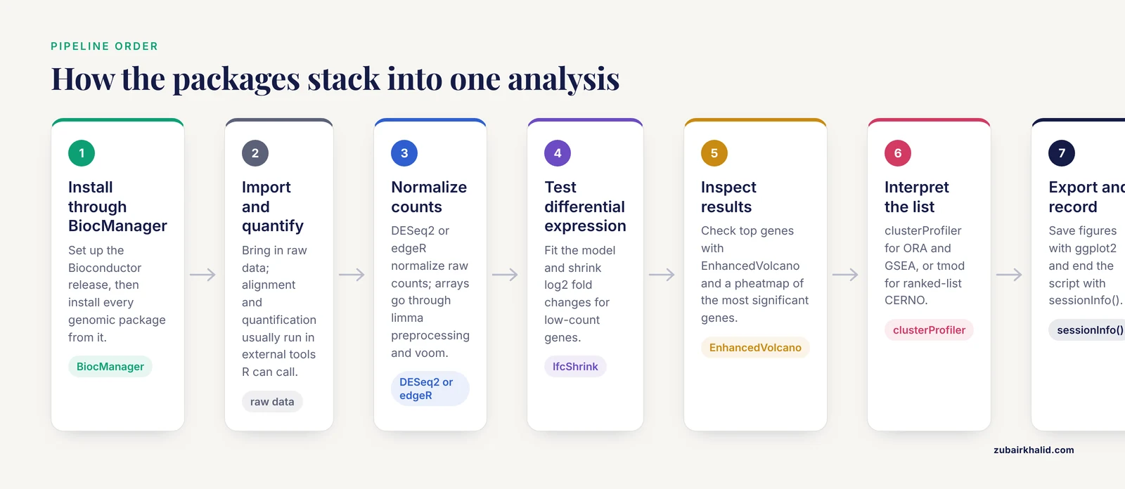
Individual packages are tools. The skill beginners actually need is assembling them into a pipeline where each step's output feeds the next. A verified miRNA-seq workflow built in R shows the full arc: raw data preprocessing, quality control, alignment, quantification, normalization, differential expression analysis, target prediction, functional enrichment, and regulatory network construction, with species-specific annotation and modular customization so researchers can swap components, and with network visualization handed off to Cytoscape [4]. MicroRNAs, or miRNAs, are short regulatory RNAs that tune gene expression after transcription.
Map that arc onto the top 10 and a generic expression project looks like this:
- Install and load everything through BiocManager.
- Import and inspect raw data, and run alignment and quantification in external tools or through R interfaces to them.
- Normalize counts with DESeq2 or edgeR, or preprocess arrays and apply voom with limma.
- Test differential expression and shrink fold changes.
- Inspect results with EnhancedVolcano and pheatmap.
- Interpret with clusterProfiler for ORA and GSEA, or tmod for ranked-list CERNO.
- Export figures with ggplot2 and record the session with sessionInfo().
The same skeleton transfers to miRNA biomarker discovery, disease modeling, and integrative multi-omics studies, which is why the miRNA-seq protocol was written as a modular R workflow rather than a fixed script [4].
Pros and Cons: Choosing Between Packages That Overlap
The hardest beginner question is not which package to learn first, it is which of two similar packages to trust. Here is how the overlaps actually resolve.
DESeq2 vs edgeR vs limma-voom
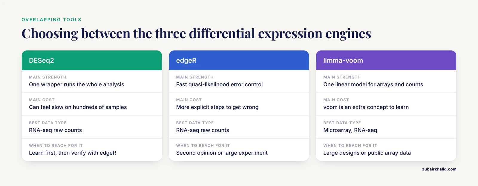
DESeq2 pros: a single wrapper function runs the whole analysis, defaults are sensible, log2 fold changes are shrunk toward zero for low-count genes, and the community documentation is the largest of the three. Cons: it can feel slow on experiments with hundreds of samples, and strong defaults can hide decisions you should be making consciously.
edgeR pros: fast, with a quasi-likelihood testing framework built for tight error rate control, plus fine-grained control over dispersion estimation and model terms. Cons: more explicit steps mean more places to go wrong, and you will read more of the vignette before your first result.
limma-voom pros: one linear model framework covers microarrays and RNA-seq, precision weights handle genes whose variance depends on expression level, and it is the fastest of the three on large designs. Cons: the voom transformation is an extra concept to learn, and very small experiments leave less information for the empirical Bayes step to borrow.
A defensible default: learn DESeq2 first, verify key findings with edgeR, and move to limma-voom when sample counts grow large or arrays enter the picture.
clusterProfiler vs tmod
clusterProfiler pros: one interface to Gene Ontology, KEGG, and many other databases, both ORA and GSEA, and utilities such as compareCluster that test several gene lists side by side. Cons: results depend on annotation versions and a correctly specified gene universe, and the breadth of options can overwhelm a first analysis.
tmod pros: fast ranked-list testing with a reproducibility pedigree, minimal tuning, and a simple CRAN install [3]. Cons: its built-in gene set collections are narrower than the database sweep clusterProfiler offers, and it is a specialist tool rather than a full enrichment suite.
Practical rule: report ORA and GSEA from clusterProfiler as your primary analysis, and reach for tmod's CERNO test when reproducibility across related datasets is the priority, which is the setting the algorithm was benchmarked for [3].
ggplot2 vs base graphics vs pheatmap
Base R graphics come free and are fine for quick looks. ggplot2 earns its learning curve the moment a figure needs a legend you did not fight for. pheatmap is a specialist that saves you an hour of hand-rolled clustering code in ggplot2. Use all three without guilt.
Worked Scenarios: Three Beginner Projects
Scenario 1: Bulk RNA-seq, treated versus control
Six samples, three versus three, a count matrix from your core facility. Load counts with DESeqDataSetFromMatrix, include batch in the design if sequencing ran in two batches, run DESeq, extract results, and shrink fold changes. Check the top genes with EnhancedVolcano and a pheatmap of the 30 most significant genes. Finish with enrichGO on the significant list, universe set to all detected genes. Packages touched: BiocManager, DESeq2, EnhancedVolcano, pheatmap, clusterProfiler, ggplot2. That is a complete, defensible first analysis.
Scenario 2: A public microarray dataset
You found an expression dataset from a published study and want to reanalyze it. Bioconductor protocols describe exactly this path for public array data, from probe-level preprocessing through differential expression and coexpression networks [1]. limma handles the linear model, and the platform-specific Bioconductor packages handle preprocessing. Because arrays report continuous intensities rather than counts, you skip voom and model log-intensities directly.
Scenario 3: A ranked list and a reproducibility requirement
Your lab combines expression data from related studies and needs enrichment results that hold up across datasets. Skip cutoff-based ORA and feed each study's full ranked list to tmod's CERNO test, which was developed and benchmarked for precisely this setting [3]. If collaborators do not use R, point them to the tmod.online implementation of the same algorithm [3].
Specialized Packages Worth Knowing After the Top 10
Once the core ten feel comfortable, three specialized packages show how far R reaches, and each wraps an entire workflow rather than a single statistical test.
COPS targets multi-omic disease subtype discovery. It evaluates single-view and multi-view clustering results using similarity networks, kernel methods, dimensionality reduction, and pathway knowledge integration, then scores outcomes on clustering agreement with the Adjusted Rand Index, a similarity score between clusterings, on survival relevance through Cox regression models with relevant covariates, and on stability, with cross-fold validation built in. Its published evaluation contrasted data-driven and pathway-driven clustering across seven cancer types, including breast, prostate, and lung, using mRNA, copy number variation, miRNA, and DNA methylation data [5]. Install it when subtyping is the goal, not before.
longreadvqs implements the QoALa workflow for comparing viral quasispecies, the constantly mutating mixtures of related viral variants within a host, from long-read sequencing data. The workflow minimizes position-wise noise in read alignments, standardizes sample sizes, and compares diversity across related samples with integrated visualization. Benchmarking on simulated SARS-CoV-2 and HIV-1 datasets showed better recovery of quasispecies composition than existing error-correction methods, particularly in preserving nucleotide diversity and hierarchical population structure, and real data from five studies covering HCV, HBV, HIV-1, SARS-CoV-2, and influenza A on major long-read platforms demonstrated the workflow's range [6].
Cogito gives an unbiased, structured overview of complex genomic datasets that mix data types, for example RNA-seq and ChIP-seq, across multiple conditions. It compares annotated genomic intervals systematically, produces a text-based report plus customizable visualizations, and is designed to surface correlations you might otherwise miss, or keep you from overrating one, before you commit to a full reanalysis [7].
The lesson from all three: once you know the core packages, learning a new one is mostly learning its data format, not a new language.
Common Mistakes and Limitations
These errors cost beginners the most time, listed in the order they usually strike.
- Feeding normalized values into DESeq2 or edgeR. Both expect raw integer counts and perform their own normalization. TPM and FPKM columns, which are expression values scaled by gene length and library size, will produce confident nonsense.
- Reading raw p values as significance. With 20,000 genes tested, hundreds will show p < 0.05 by chance alone. Report FDR-adjusted values, where FDR stands for false discovery rate, the expected proportion of false positives among your calls.
- Using the wrong gene universe in ORA. The background should be every gene your experiment could have detected, typically all genes with nonzero counts, not the whole genome.
- Hiding batch effects instead of modeling them. If treated samples were sequenced on a different day than controls, the design formula needs the batch term, or your results describe the sequencer rather than the biology.
- Trusting a heatmap as a test. Hierarchical clustering is sensitive to scaling and distance choices. A striking cluster is a hypothesis, and you confirm it with statistics.
- Not recording the environment. Call sessionInfo() at the end of every script, set a seed with set.seed() before any stochastic step, and keep one project per directory. Version records are what make an analysis rerunnable years later.
- Copy-pasting design formulas. The design argument is your statistical model. A formula you do not understand produces a result you cannot defend.
- Expecting one package to be the pipeline. Even the best package covers one step. The miRNA-seq protocol cited above integrates many packages and still hands network visualization to Cytoscape [4].
Limitations, stated plainly. Packages change, so a script that ran last year may need updates after a Bioconductor release. Statistical significance is not biological importance, and a low FDR on a pathway containing three genes deserves skepticism. Individual research questions, like individual patients in a clinical setting, need expert judgment on study design and interpretation, which no package checklist replaces.
Frequently Asked Questions
Do I need to know R programming before using these packages?
No, but you need the basics. Variables, data frames, and function calls are enough to run a full DESeq2 analysis, and you will pick up more as you go. Budget a weekend for an introductory R course, then learn by rerunning a published workflow rather than by reading a language manual cover to cover.
What is the difference between CRAN and Bioconductor?
CRAN is the general R archive for packages of all kinds, while Bioconductor is a genomics-specific repository with shared data structures and coordinated twice-yearly releases. Install CRAN packages with install.packages() and Bioconductor packages with BiocManager::install(). Both are free and open source.
Should beginners learn DESeq2 or edgeR first?
Learn DESeq2 first. Its single-function wrapper and strong defaults get you to a correct result with fewer decisions, and its documentation is the most beginner-friendly of the count-based tools. Add edgeR when you want a second opinion, a large experiment, or finer control over the statistical model.
Which package should I use for gene set enrichment?
Use clusterProfiler when you have a gene list and want over-representation analysis or GSEA against major databases. Use tmod when you have a ranked list and reproducibility across datasets is the priority, because its CERNO algorithm was built and benchmarked for that setting [3]. Many projects use both.
Can a complete analysis run in R alone?
Almost. Statistics, normalization, enrichment, and figures run entirely in R, and verified R workflows exist for full pipelines from raw preprocessing through network construction. Raw sequence alignment and quantification usually run in external tools that R can call, and network visualization often moves to Cytoscape.
How do I keep my analysis reproducible?
Write scripts instead of clicking, record package versions with sessionInfo(), set a random seed before stochastic steps, and install packages through BiocManager so versions trace to a named Bioconductor release. Keep one project per directory and archive the raw data alongside the code.
Sources
- The use of open source bioinformatics tools to dissect transcriptomic data.
- Genes and Gene Functions Associated with Morphological, Productive, Reproductive, and Carcass Quality Traits in Pigs: A Functional Bioinformatics Approach.
- Gene set enrichment for reproducible science: comparison of CERNO and eight other algorithms.
- A Verified Workflow for MiRNA-Seq Data Processing and Bioinformatics Analysis Using R.
- COPS: A novel platform for multi-omic disease subtype discovery via robust multi-objective evaluation of clustering algorithms.
- QoALa: A comprehensive workflow for viral quasispecies diversity comparison using long-read sequencing data.
- Cogito: automated and generic comparison of annotated genomic intervals.