How to Download All Genomes for a Taxonomic Group from NCBI Datasets
By Dr. Zubair Khalid, DVM, MS, PhD ·

By the end of this guide you will be able to download all genomes for any taxonomic group, from a single species to an entire genus or family, directly from NCBI Datasets using the official datasets command-line tool. You will also learn how to filter those genomes by assembly level and release date, convert the metadata into a spreadsheet-friendly table, verify the download is complete, and pick the right method when the taxon contains tens of thousands of assemblies.
To follow along you need a Linux, macOS, or Windows (WSL) machine with a terminal, roughly 10 to 100 GB of free disk space depending on the taxon, and either Conda or the ability to download a binary file. No account or API key is required for the standard download commands shown here.
NCBI maintains the largest public archive of genome assemblies in the world, and large-scale reanalysis projects routinely pull thousands of datasets from it. One recent metagenomics pipeline, for example, automatically downloaded more than 16,000 human gut metagenome samples from the Sequence Read Archive and profiled them on a high-performance cluster in under 55 hours, download time included [1]. The same pattern shows up across the literature. A wastewater resistome study in Türkiye downloaded ten metagenomes from the NCBI SRA database, assembled them, and reconstructed high-quality metagenome-assembled genomes for downstream analysis [2]. Whether you work with isolates, metagenome-assembled genomes, or raw reads, the first practical step is always the same: get the sequence data off NCBI and onto your own machine. This guide covers that step for whole-genome assemblies.
Why Download Genomes Rather Than Fetch Reads
Many analyses need reference genomes on local disk, not raw reads from the sequencing archive. Building a BLAST database, running a pangenome analysis with tools like Panaroo or Roary, constructing a phylogeny, or screening for antimicrobial resistance genes all require FASTA files you control locally. Mapping metagenomic reads against a local, non-redundant reference set is also far less computationally intensive than mapping every read against a massive central database such as NCBI's nt, which is why profiling tools deliberately subsample or restrict the reference space [3].
Whole-genome approaches have become a standard part of comparative genomics for exactly this reason. Alignment-free phylogenetic methods, for instance, estimate evolutionary distances from complete genomes directly, and researchers validated such methods against the NCBI taxonomy across hundreds of bacterial and archaeal genomes [4]. Those workflows all begin with the same practical problem: obtaining a complete, consistent set of genome files for the organisms of interest.
How NCBI Datasets Organizes Genome Data
Before running commands, understand what you are downloading. NCBI stores genome assemblies in two related archives, and the difference matters for reproducibility.
GenBank (GCA accessions). The community archive. Submitters deposit assemblies here. Every assembly submitted to INSDC members ends up in GenBank with an accession beginning with GCA.
RefSeq (GCF accessions). NCBI's curated, non-redundant subset. A RefSeq assembly is typically derived from a corresponding GenBank entry, has been through NCBI's annotation and quality pipelines, and carries an accession beginning with GCF. Most GenBank assemblies for the same organism have a RefSeq counterpart, so a naive download of everything will often give you two copies of nearly the same genome.
Assembly levels. Each assembly is tagged as complete (a finished genome, often in one sequence per chromosome), chromosome (assembled to chromosome scale with gaps), scaffold, or contig. These labels describe how fragmented the assembly is, not whether it is biologically correct.
NCBI Datasets. A service on top of these archives, exposed in three ways: the web interface at the NCBI Datasets site, the datasets and dataformat command-line tools, and a programmatic API via the ncbi-datasets-pylib Python package. The CLI is the workhorse for the phrase most people actually search for, "download all genomes for a taxonomic group NCBI Datasets," because it resolves a taxon name to every matching assembly automatically.
If you have previously used NCBI through the older E-utilities endpoints or the Entrez Direct tools, you can still accomplish this workflow that way, but the Datasets CLI does the accession resolution, package assembly, and metadata handling for you in one step. It is the recommended entry point in any modern NCBI databases guide for bulk genome retrieval.
Install and Set Up the Tools
Install with Conda if you use an environment manager.
conda install -c conda-forge ncbi-datasets-cliAlternatively, download the official static binaries directly from the NCBI FTP server.
curl -o datasets "https://ftp.ncbi.nlm.nih.gov/pub/datasets/command-line/v2/linux-amd64/datasets"
curl -o dataformat "https://ftp.ncbi.nlm.nih.gov/pub/datasets/command-line/v2/linux-amd64/dataformat"
chmod +x datasets dataformat
mkdir -p ~/bin && mv datasets dataformat ~/bin/
export PATH="$HOME/bin:$PATH"
For macOS, replace linux-amd64 with mac-arm64 on Apple Silicon or mac-amd64 on Intel machines. On Windows, run these commands inside WSL.
You will also want unzip (usually preinstalled) and jq for JSON handling, which you can install with conda install -c conda-forge jq.
Verify the installation.
datasets --version
dataformat --version
Expected output looks like this (your version numbers will differ).
datasets: 16.38.0
dataformat: 16.38.0
If datasets: command not found appears, the binary is not on your PATH. Either add the containing directory to PATH as shown above or call the binary by its full path.
Step-by-Step Walkthrough: Download All Genomes for a Species
The worked example below uses Listeria monocytogenes, a species with a manageable number of assemblies, so you can follow the logic before scaling up. Every command generalizes to any taxon name.
Step 1: Resolve the taxon name and get the NCBI Taxonomy ID
Taxon names change as taxonomy is revised, so anchor your analysis to a stable numeric Taxonomy ID where possible. Ask Datasets to resolve the name.
datasets summary taxonomy taxon "Listeria monocytogenes" --as-json \
  | jq '.reports.taxonomy | {tax_id, scientific_name, rank}'
Expected output (abbreviated).
{
  "tax_id": "169963",
  "scientific_name": "Listeria monocytogenes",
  "rank": "species"
}
Record this ID. If a paper or a colleague later asks exactly which set of genomes you used, the Taxonomy ID plus the download date pins it down unambiguously.
Step 2: Preview the download before committing
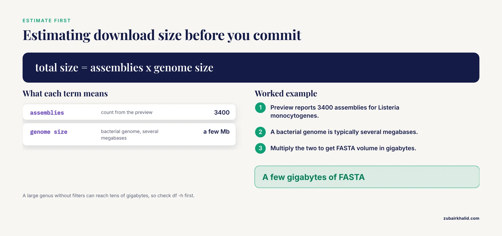
Never download blind. Ask Datasets how many assemblies match your taxon and what the filters would select.
datasets summary genome taxon "Listeria monocytogenes" --as-json \
  | jq '{total_count, reports: (.reports | length)}'
Expected output (abbreviated, counts will change as new assemblies are released).
{
  "total_count": 3400,
  "reports": 3400
}
You can also list the first few accessions to sanity-check what you are about to pull.
datasets summary genome taxon "Listeria monocytogenes" --as-json \
  | jq '.reports[0:5] | .[].accession'
Expected output (abbreviated).
"GCF_000196035.1"
"GCA_000196135.1"
"GCA_000168175.1"
"GCA_000836265.1"
"GCA_000620665.1"
The human-readable summary without -as-json is also useful because it reports how many assemblies are RefSeq versus GenBank and how many are marked as reference.
datasets summary genome taxon "Listeria monocytogenes"Abbreviated illustrative output.
Number of Genomes:
3,400

For filtering:
	Reference: 2
	GenBank: 3,250
	RefSeq: 150
This preview step is where you decide how big the download will be. Listeria monocytogenes has thousands of assemblies, a bacterial genome is typically several megabases, so a full set of FASTA files alone will run to a few gigabytes. A large genus such as Streptococcus or Enterobacter can run to tens of gigabytes. Estimate before you commit.
Step 3: Choose your filters
The most common mistake is downloading everything when you need a well-defined subset. Datasets exposes the filters that matter as command-line flags, and the following table summarizes them.
| Flag | What it controls | Useful values |
|---|---|---|
| , - | , - | , - |
taxon (positional) | Any scientific name, common name, or Taxonomy ID | "Listeria monocytogenes", 169963 |
-assembly-level | Fragmentation of assemblies | complete, chromosome, scaffold, contig |
-reference | Only assemblies flagged as reference or representative | (no value) |
-annotated | Only assemblies with NCBI annotation | (no value) |
-released-on-or-after | Restrict to assemblies released after a date | 2020-01-01 |
-exclude-atypical | Drop assemblies flagged atypical in assembly metadata, such as metagenome-derived or heavily contaminated entries | (no value) |
-include | Which file types land in the package | genome, gbff, gff3, protein, rna, cds, gtf, seq-report, none |
-filename | Name of the output zip | listeria.zip |
Run datasets download genome, help to see the full, current list on your installed version, since flags are added between releases.
A sensible default for most comparative analyses is one genome per species or strain lineage with annotation, excluding atypical entries. For Listeria monocytogenes that means dropping the massive GenBank collection of near-duplicate strains and taking the RefSeq set.
Step 4: Run the download
Download the RefSeq genomes with nucleotide FASTA and GenBank flat files included.
datasets download genome taxon "Listeria monocytogenes" \
  --annotated \
  --exclude-atypical \
  --include genome,gbff,seq-report \
  --filename listeria_refseq.zip
Expected terminal output (abbreviated).
Downloading: ncbi_dataset.zip    100.0%
Packages: 1 total, 1 downloaded (150 genome packages)
Each flag does specific work. -annotated filters to assemblies NCBI has annotated, which matters if you plan to extract genes or proteins. -exclude-atypical removes assemblies flagged as atypical, which is your main defense against accidentally including metagenome-derived contig soup in an isolate-based analysis. -include genome,gbff,seq-report requests the nucleotide FASTA, the GenBank-format annotation file, and the per-assembly sequence report, and skips the larger protein, CDS, and GFF3 bundles you may not need. -filename controls the output name. Omit it and Datasets writes ncbi_dataset.zip in the current directory.
If you instead want absolutely every assembly for the taxon, both archives, drop -annotated and add -assembly-level choices explicitly.
datasets download genome taxon "Listeria monocytogenes" \
  --assembly-level complete \
  --include genome \
  --filename listeria_all_complete.zip
-assembly-level complete restricts to finished assemblies, which for many species reduces the set from thousands to a handful.
Step 5: Unzip and inspect the package
unzip listeria_refseq.zip -d listeria_refseq
ls listeria_refseq/ncbi_dataset/data/
Expected output (abbreviated).
GCF_000196035.1  GCF_000836265.1  assembly_data_report.jsonl
GCA_000168175.1  dataset_catalog.json
Each accession becomes a directory. Inside an assembly directory you will find files like GCF_000196035.1_ASM196v1_genomic.fna for the sequence and GCF_000196035.1_ASM196v1_genomic.gbff for the annotated record. The assembly_data_report.jsonl file at the top level holds one JSON line of metadata per genome and is the key to verification and downstream filtering.
Step 6: Convert the metadata to a table
dataformat tsv genome info \
  --inputfile listeria_refseq/ncbi_dataset/data/assembly_data_report.jsonl \
  --fields accession,organism-name,organism-infraspecific-names-strain,assembly-level,assembly-stats-contig-n50,source-database \
  --output listeria_summary.tsv
head -4 listeria_summary.tsv
Expected output (abbreviated).
Accession	Organism Name	Strain	Assembly Level	Contig N50	Source
GCF_000196035.1	Listeria monocytogenes	1/2a F2365	Chromosome	2,944,084	RefSeq
GCF_000836265.1	Listeria monocytogenes	10403S	Contig	1,076,395	RefSeq
GCA_000168175.1	Listeria monocytogenes	J0161	Chromosome	2,944,084	GenBank
Run dataformat tsv genome info, help to see every field token available on your version. You can request genome size, biosample accession, release date, assembly statistics, and dozens of other fields, and open the result directly in a spreadsheet or R.
Step 7: Verify the download
Three quick checks catch most problems.
# Count the assembly directories
ls -d listeria_refseq/ncbi_dataset/data/GC* | wc -l

# Count the metadata lines, which must match
wc -l listeria_refseq/ncbi_dataset/data/assembly_data_report.jsonl

# Confirm every FASTA exists and is nonempty
find listeria_refseq/ncbi_dataset/data -name "*_genomic.fna" -size -1k
Expected output.
150
150
(no output, meaning no suspiciously small files)
If the directory count equals the JSONL line count equals the number reported in your Step 2 preview, the package is internally consistent. The find command returning nothing confirms no truncated FASTA files. For FTP downloads, which we cover below, NCBI provides an md5sums.txt in each assembly directory, and md5sum -c verifies them.
Step 8: Scale up with a genus or family
The same command pattern works at any rank. To pull the complete assemblies for the whole genus Vibrio:
datasets summary genome taxon "Vibrio" --as-json | jq '.total_count'
datasets download genome taxon "Vibrio" \
  --assembly-level complete \
  --include genome \
  --filename vibrio_complete.zip
The taxon resolver walks down the taxonomy tree from the name you give it, so a family name selects every species and strain below it. This is the core of how to use NCBI efficiently for bulk retrieval: one command, any rank, everything underneath included.
Step 9: Alternative route for very large taxa, the genome FTP
When a taxon contains tens of thousands of assemblies, the Datasets zip can exceed practical limits for web and API delivery, and the flat FTP layout is often more efficient because you fetch only the files you need. NCBI publishes a machine-readable catalog of every RefSeq assembly.
wget https://ftp.ncbi.nlm.nih.gov/genomes/refseq/assembly_summary_refseq.txtThis tab-delimited file lists every RefSeq assembly with the organism name in column 8, the Taxonomy ID in column 6, the assembly level in column 12, and the FTP path in column 20. Build a list of FASTA URLs for one species and fetch them.
awk -F'\t' 'NR>2 && $8=="Listeria monocytogenes" {print $20}' \
  assembly_summary_refseq.txt \
  | sed 's|^ftp://|https://|' \
  | awk '{print $0 "/" $NF "_genomic.fna.gz"}' \
  > fna_urls.txt

wc -l fna_urls.txt
wget -i fna_urls.txt
The first awk selects rows for the species and prints the FTP path, the sed converts to the HTTPS mirror, and the second awk appends the standard FASTA filename, which is the assembly directory name followed by _genomic.fna.gz. Swap $8 for $6==169963 to filter by Taxonomy ID instead, or add $12=="Complete" to restrict to finished assemblies. Each assembly directory on the FTP server contains an md5sums.txt file you can use for verification.
Tips for Reliable, Reproducible Bulk Downloads
Preview twice, download once. Run datasets summary with the exact flags you intend to use before adding -filename. The count in the summary tells you what the download will contain, and it is the number your verification step must reproduce.
Freeze your accession list. NCBI gains new assemblies continuously. For reproducibility, save the accession list from your summary to a text file and use it for repeat downloads.
datasets summary genome taxon "Listeria monocytogenes" --as-json \
  | jq -r '.reports[].accession' > listeria_accessions.txt

datasets download genome accession --inputfile listeria_accessions.txt \
  --include genome --filename listeria_frozen.zip
This guarantees that a collaborator re-running the download next year gets the same set of assemblies, because the set is now defined by accessions rather than by whatever NCBI contains at download time.
Keep the zip, not the unzipped tree. On shared and networked filesystems, tens of thousands of small files per directory tree degrade performance. Keep the zip archive on long-term storage and unzip only what an individual job needs.
Minimize -include. Every file type you add multiplies download size. Nucleotide FASTA (genome) is usually sufficient for mapping and pangenome tools. Add protein or gbff only when the analysis actually consumes them.
Use -no-progressbar in scripts. Progress rendering adds overhead and clutters logs. Any Datasets command run inside a batch script or Nextflow process should carry it.
Match the download method to the scale. One recent large-scale reanalysis project downloaded and profiled 16,462 metagenome samples from the SRA in under 55 hours on a cluster, and the authors explicitly designed the pipeline to accept accession and study identifiers as input [1]. The lesson generalizes: at four-figure dataset counts, drive downloads from a saved list of identifiers inside a pipeline, not from interactive commands.
Common Mistakes and Limitations
Downloading GenBank and RefSeq copies of the same genome. Most RefSeq assemblies have a GenBank twin. If you download both archives, your pangenome or phylogeny will contain near-identical duplicate tips. Decide up front. For most analyses, take RefSeq only, or take GenBank only when RefSeq coverage for your group is thin.
Assuming "complete" means what you think it means. The assembly level complete describes contiguity, not curation quality. A complete assembly can still carry plasmids, contamination, or annotation errors. Read the assembly metadata rather than trusting a single field.
Letting the taxon name do too much work. A genus-level query like taxon "Bacillus" selects every species NCBI places under that genus today. Taxonomy is revised regularly, so a name-based query executed this month may return a different set than the same query last year. Prefer Taxonomy IDs for anything you will repeat.
Mixing metagenome-assembled genomes with isolate genomes. Assembly metadata lets you tell them apart, and -exclude-atypical filters many of them out. Studies that reconstruct MAGs from metagenomes, such as the wastewater resistome reanalysis that assembled high-quality MAGs from NCBI SRA data [2], treat MAGs as a distinct category precisely because their quality statistics and provenance differ from isolate assemblies. Failing to separate them is a silent analysis error.
Ignoring disk and inode limits. A full genus can mean 10,000 or more directories, each holding several files. Check available space with df -h before a large download, and note that some shared filesystems enforce per-directory file-count limits that unzip will hit mid-extraction.
Treating NCBI annotation as the only annotation. NCBI records are authoritative for sequence and assembly metadata, but specialized model-organism databases frequently carry richer functional annotation than the corresponding NCBI records, a difference noted explicitly in the documentation of curated resources such as the Chinchilla Research Resource Database [5]. If your analysis depends on gene function calls, cross-check against the relevant community database for your organism.
Not planning for taxonomy drift in long projects. Reference sets you build today will not automatically include assemblies released later, and NCBI may reassign taxa. Re-run your summary periodically, diff the accession list against your frozen copy, and document every update.
Overwriting downloaded data. datasets download writes a fresh zip each time. Version your output directories by date and accession-list hash so an accidental re-download does not destroy a verified dataset.
Choosing the Right Download Method: Web Interface, Datasets CLI, FTP, and the Python Library Compared
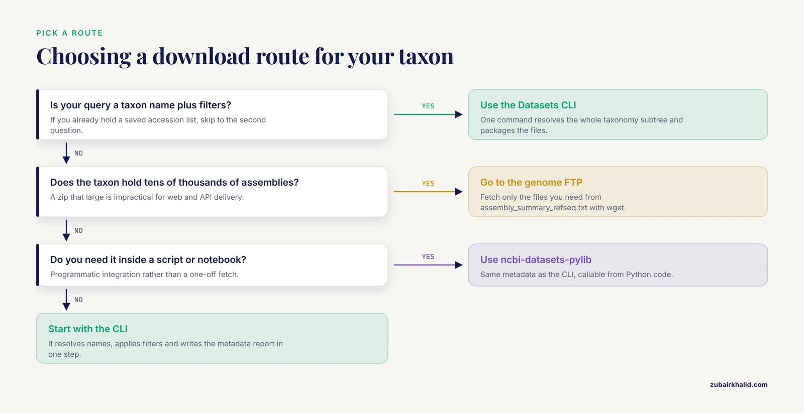
The walkthrough in the main guide centers on the datasets CLI, and for good reason: it resolves taxon names, applies filters, and packages files in a single command. But it is not the only route, and picking the wrong route for your situation wastes hours. Here is an honest comparison of the four practical options.
| Method | Best for | Strengths | Weaknesses |
|---|---|---|---|
| NCBI Datasets web interface | One-off downloads, exploratory browsing | No installation, clickable filters, immediate | Not scriptable, impractical past a few hundred assemblies, no reproducibility trail |
datasets CLI | Taxon-driven downloads up to thousands of assemblies | One command resolves the whole taxonomy subtree, filters built in, metadata report included | Zip size limits on very large taxa, requires installation |
Genome FTP and assembly_summary_refseq.txt | Tens of thousands of assemblies, selecting individual file types | Fetch only what you need, checksums available, works with wget and rsync | You resolve the taxon yourself, file naming conventions require care |
ncbi-datasets-pylib Python package | Programmatic and pipeline integration | Fits inside scripts and notebooks, same metadata as the CLI | Learning curve, less community troubleshooting material available |
A fifth route, the older E-utilities or Entrez Direct tools, still works and remains useful when you need Entrez queries the Datasets API does not express, but for the specific task of "give me every assembly under this taxon" it requires you to write the accession resolution loop that Datasets does for you. Treat it as a fallback, not a starting point.
Two decision rules cover most cases. First, if your query is "taxon name plus filters," use the CLI. Second, if your query is "a saved list of accessions, each needing only one file type," the FTP route with a URL list is usually faster and more restartable, because wget -c resumes an interrupted fetch of a single large file, which the zip-based CLI does not do. You can mix methods within one project: freeze your accession list with the CLI, then fetch individual FASTA files over HTTPS.
A Second Worked Example: Building a Family-Level Reference Set in Batches
The main guide shows a single-shot species download. Real projects rarely stop there. Suppose you need every available assembly for the genus Mycoplasma, and the preview tells you there are far too many to fetch in one zip. This is the pattern to use.
Start by freezing the accession list, exactly as the tips section recommends.
datasets summary genome taxon "Mycoplasma" -as-json \
  | jq -r '.reports[].accession' > mycoplasma_all.txt

wc -l mycoplasma_all.txt
Assume the count is several thousand. Split the list into manageable chunks. Five hundred accessions per chunk keeps each zip a reasonable size for a species with small genomes, and you should adjust the chunk size downward for large genomes.
split -l 500 mycoplasma_all.txt myco_chunk_
ls myco_chunk_*
Now loop over the chunks, downloading each as its own zip. This is where -no-progressbar earns its place, because the loop produces clean logs you can grep later for failures.
for f in myco_chunk_*; do
  datasets download genome accession -inputfile "$f" \
    -include genome \
    -filename "${f}.zip" \
    -no-progressbar
done
Unzip each archive into its own directory, then merge the metadata reports so you end up with one JSONL file covering the entire genus.
for z in myco_chunk_*.zip; do
  unzip -q "$z" -d "${z%.zip}"
done

cat myco_chunk_*/ncbi_dataset/data/assembly_data_report.jsonl \
  > mycoplasma_all_reports.jsonl

wc -l mycoplasma_all_reports.jsonl
The final line count must equal the original wc -l on mycoplasma_all.txt. If it does not, some chunk failed. Re-run the loop with a guard so only missing or empty archives are retried.
for f in myco_chunk_*; do
  zip_file="${f}.zip"
  if [ ! -s "$zip_file" ]; then
    datasets download genome accession -inputfile "$f" \
      -include genome -filename "$zip_file" -no-progressbar
  fi
done
This chunked pattern has a second benefit: if your connection drops at chunk 7 of 14, you have six verified chunks on disk already and only rerun the remainder. Compare that to a single monolithic zip, where an interruption costs you the whole download.
Practical Filter Recipes for Real Analyses
The flags table in the main guide lists what each option does. This section shows how to combine them for the situations that actually come up.
Recipe 1: A current snapshot of a species for variant or gene presence work. You want recent, annotated, isolate-derived assemblies.
datasets download genome taxon 169963 \
  -annotated \
  -exclude-atypical \
  -released-on-or-after 2022-01-01 \
  -include genome,gbff \
  -filename listeria_recent_annotated.zip
Using the Taxonomy ID instead of the name makes the command rerunnable, and the date filter caps the size while capturing anything new since your last update.
Recipe 2: A reference panel for a phylum-level survey. You want one curated genome per species, not a strain collection.
datasets download genome taxon "Firmicutes" \
  -reference \
  -include genome,seq-report \
  -filename firmicutes_ref.zip
The -reference flag restricts to reference and representative assemblies, which converts an impossible download into a tractable one. Note that representative coverage is uneven across understudied groups, so check the resulting count before building assumptions on it.
Recipe 3: Only finished genomes for a structural or synteny analysis. Closed genomes matter when order and orientation of sequences must be trusted.
datasets download genome taxon "Salmonella enterica" \
  -assembly-level complete \
  -include genome,gbff \
  -filename salmonella_complete.zip
Recipe 4: Filtering after download. Sometimes the CLI flags cannot express what you need, such as an assembly statistic threshold. In that case, download with seq-report, convert to TSV, and filter with standard text tools.
dataformat tsv genome info \
  -inputfile reports.jsonl \
  -fields accession,organism-name,assembly-level,assembly-stats-contig-n50,assembly-stats-total-sequence-length,source-database \
  -output all.tsv

awk -F'\t' 'NR==1 || $4 > 50000' all.tsv > filtered.tsv
The awk keeps the header plus every row whose contig N50 exceeds 50 kb. You chose that threshold, it is not an NCBI standard, and it should be documented in your methods. Post-hoc filtering on the TSV is more flexible than the CLI filters, at the cost of having already downloaded everything, so budget accordingly.
Turning the Metadata Report into Analysis-Ready Tables in Python and R
The assembly_data_report.jsonl file is one JSON object per line, which makes it trivially loadable in any scripting language. This is often the fastest path from download to figure.
In Python, with nothing beyond the standard library plus pandas:
import json
import pandas as pd

rows = []
with open("listeria_refseq/ncbi_dataset/data/assembly_data_report.jsonl") as fh:
    for line in fh:
        rows.append(json.loads(line))

df = pd.json_normalize(rows)
df.to_csv("listeria_metadata.csv", index=False)
print(df.shape)
Because JSONL is flat, a corrupted or partial line shows up immediately as a parse error on a specific line number, which is a useful side effect: the line count is your verification check, and the content of each line is self-describing.
In R:
library(readr)
meta <- read_tsv("listeria_summary.tsv")
summary(meta$`Contig N50`)
table(meta$`Assembly Level`, meta$Source)
Two habits pay off here. First, always regenerate the TSV from the JSONL in the same command that produces the table, so the metadata cannot silently drift from the FASTA files on disk. Second, record the exact -fields string you used. The available field tokens expand between releases, and a published table should state which tokens populated which columns. Run dataformat tsv genome info -help on your installed version for the authoritative list.
The same metadata supports decisions no single CLI filter captures. Sorting by release date reveals when a taxon's assembly effort accelerated. Cross-tabulating assembly level against source database exposes how much of a taxon exists only in GenBank. Counting distinct strain names against total assemblies gives you a rough duplication sense before you ever run a dereplication step.
Post-Download Quality Screening Before Any Analysis
Downloading is not accepting. Before genomes enter a pangenome, phylogeny, or database build, screen the set. These checks take minutes and catch problems that otherwise surface days later as unexplainable outliers.
Size and fragmentation sanity check. Use the TSV from the previous section. For bacteria, most assemblies of a given species cluster tightly in total sequence length; outliers far from the median often indicate contamination, heavy fragmentation, or mislabeled taxonomy. Print a quick distribution:
tail -n +2 listeria_summary.tsv | cut -f5 | sort -n | awk '
  {a[NR]=$1}
  END {print "n="NR, "min="a[2], "median="a[int(NR/2)], "max="a[NR]}'
Duplicate detection by strain and assembly. Sort by strain name in the TSV and look for repeated values across different accessions. Near-identical duplicates are the RefSeq GenBank twin problem caught early, and catching them before a phylogeny saves you from near-zero branch lengths that dominate the tree.
Separating MAGs from isolates. Assemblies reconstructed from metagenomes carry different provenance and quality characteristics from isolate assemblies, which is why MAG-focused studies treat them as a distinct category throughout their workflows [2]. The -exclude-atypical flag removes many atypical entries at download time, but scan the remaining metadata for infraspecific names or assembly-level patterns that suggest environmental reconstruction rather than clonal culture, and drop or tag them explicitly.
Annotation completeness. If you downloaded gbff or protein files, confirm the counts line up. An assembly directory with a FASTA but no annotation file either was not annotated or was filtered inconsistently. Decide per genome whether to proceed, reannotate locally, or exclude, and record the decision.
Checksum verification for FTP-sourced files. For anything pulled over FTP or HTTPS from the FTP mirror, verify against the md5sums.txt shipped in each assembly directory:
cd <assembly_directory>
md5sum -c md5sums.txt
Any failure means a truncated transfer. Re-fetch that single file rather than the whole set. Screen your assembly metadata rather than trusting any single field, because contiguity labels and quality flags describe different things and a set can pass one check while failing another.
Feeding Downloaded Genomes into Common Downstream Workflows
The download is a means to an end. Here is how the package contents map onto the analyses that motivate most bulk downloads, with the file-type choices that make each workflow smooth.
Building a local BLAST database. The nucleotide FASTA files are sufficient. Concatenate them into one file with per-genome sequence headers preserved, then build the database:
cat listeria_refseq/ncbi_dataset/data/GC*/*_genomic.fna > all_listeria.fna
makeblastdb -in all_listeria.fna -dbtype nucl -out listeria_db
Keep the TSV metadata alongside the database so a hit's accession can be traced back to strain, assembly level, and release date. A BLAST hit without that context is only half an answer.
Pangenome analysis. Tools in this space consume per-genome annotation, typically GFF3 or GenBank format, one input per genome. Download with -include gff3 or -include gbff, or reannotate all genomes locally with a single tool so that gene prediction parameters are uniform across the set. Uniformity matters more than provenance here: mixing genomes annotated years apart with different pipeline versions introduces artifacts that look like biology. If your pangenome tool requires consistent annotation, reannotation of the full set is usually safer than mixing NCBI annotation of varying vintage.
Mapping read sets against a local reference. Profiling and mapping against a curated local set is far cheaper than searching against a monolithic central database, which is why modern profilers deliberately limit their reference space [3]. For this use, dereplication is the critical post-download step. Cluster your downloaded genomes by average nucleotide identity and keep one representative per cluster, with a common practice of thresholds somewhere in the 95 to 99 percent range depending on how finely you want to resolve strains. The seq-report TSV tells you which accession within a cluster has the highest contiguity, which is usually the right representative to keep.
Phylogenetics and comparative genomics. Alignment-free methods estimate distances from complete genomes directly and were validated against the NCBI taxonomy across large bacterial and archaeal sets [4], and they consume the FASTA files exactly as downloaded. Core-gene and whole-genome alignment approaches instead need annotation or careful ortholog detection, which pulls in the protein and gff3 include types. Choose the include set based on the tree-building method before downloading, not after, because re-downloading a genus twice is exactly the kind of wasted cycle this guide exists to prevent.
Antimicrobial resistance and virulence screening. These workflows are FASTA-only and benefit from the largest practical genome count, since sensitivity rises with panel size. The RefSeq-only, -exclude-atypical download is the right starting point, and the wastewater resistome literature demonstrates the downstream pattern: assemble or retrieve genomes, screen against curated resistance databases, and report hits with assembly provenance attached [2].
Troubleshooting Guide: What Breaks and How to Fix It
datasets: command not found after Conda install. Your Conda environment is not active or the environment's bin directory is not on PATH. Run conda activate for the relevant environment and check which datasets. If you installed the static binary, confirm the move into ~/bin actually happened and that export PATH="$HOME/bin:$PATH" is in your shell profile, not just the current session.
The dataformat field token you used produces an error or an empty column. Field tokens evolve between releases. Never copy a -fields string from an old tutorial, including older versions of this guide. Run dataformat tsv genome info -help and confirm every token exists on your installed version. An empty column with no error usually means the token exists but holds no value for your assemblies, which is different from a wrong token.
A zip that will not open, or opens partially. First test integrity: unzip -t yourfile.zip. If it reports errors, the transfer was incomplete. Delete the zip and re-download. If the zip opens but a specific accession directory is missing files, fetch that single accession directly:
datasets download genome accession GCF_000196035.1 \
  -include genome,gbff -filename repair_one.zip
This one-accession pattern is also your best friend when an assembly's files turn out to be unexpectedly large, since you can inspect it in isolation before deciding whether to keep it.
An interrupted or very slow FTP fetch. Run wget with the -c flag so partial files resume rather than restart. If FTP connections stall, use the HTTPS mirror of the same paths, as the main walkthrough does with its sed substitution. For massive parallel fetches, keep concurrency modest, because hammering the mirror with dozens of simultaneous connections frequently achieves less throughput than a few sequential ones.
Unzip dies partway with a file-count or disk error. Check df -h and, on shared systems, ask your administrators about per-directory entry limits. The fix is selective extraction: unzip only the accessions your current job needs.
unzip listeria_refseq.zip "ncbi_dataset/data/GCF_000196035.1/*" -d work/Keep the original zip intact and extract on demand. This is the disk-friendly pattern the tips section recommends, and it doubles as your recovery path when a filesystem misbehaves.
Counts that do not reconcile. If ls -d data/GC* | wc -l and wc -l assembly_data_report.jsonl disagree, or either disagrees with your Step 2 preview count, something was filtered or lost in transit. The JSONL is the authoritative record of what the package intended to contain; missing directories mean transfer or extraction trouble, and a count below your preview means the download was executed with different flags than the preview.
Annotation files missing for some assemblies. Not every assembly carries NCBI annotation. If you used -annotated and still see gaps, check the metadata for those accessions. The practical fallback is local reannotation, which as noted above also solves the annotation-consistency problem for pangenome work.
Cryptic failures on very old operating systems. Static binaries avoid dependency problems, but TLS certificate bundles on aged systems can fail during HTTPS downloads. Updating the system certificate store, or running the workflow inside a current Conda environment or container, resolves most such failures without touching the tool itself.
Automation: Wrapping the Download in Scripts and Pipelines
Interactive commands are for exploration. Production downloads belong in scripts with date stamps, logs, and verification built in. A minimal shell wrapper captures the pattern:
#!/usr/bin/env bash
set -euo pipefail

TAXON_ID=169963
STAMP=$(date +%Y%m%d)
OUTDIR="downloads/${TAXON_ID}_${STAMP}"
mkdir -p "$OUTDIR"

datasets summary genome taxon "$TAXON_ID" -as-json \
  | jq -r '.reports[].accession' > "$OUTDIR/accessions.txt"

datasets download genome taxon "$TAXON_ID" \
  -annotated -exclude-atypical \
  -include genome,seq-report \
  -filename "$OUTDIR/genomes.zip" \
  -no-progressbar 2> "$OUTDIR/download.log"

unzip -q "$OUTDIR/genomes.zip" -d "$OUTDIR"

EXPECTED=$(wc -l < "$OUTDIR/accessions.txt")
ACTUAL=$(ls -d "$OUTDIR"/ncbi_dataset/data/GC* | wc -l)
if [ "$EXPECTED" != "$ACTUAL" ]; then
  echo "VERIFICATION FAILED: expected $EXPECTED, got $ACTUAL" >&2
  exit 1
fi
echo "OK: $ACTUAL assemblies in $OUTDIR"
The script records the accession list, the log, the zip, and the verification result in one dated directory. If verification fails, nothing downstream runs, because set -e stops the script. Store a checksum of the accession list alongside it:
sha256sum "$OUTDIR/accessions.txt" > "$OUTDIR/accessions.txt.sha256"For workflow managers, the same logic becomes one process or rule. Large-scale reanalysis pipelines designed for thousands of samples take accession and study identifiers as their input and drive retrieval programmatically, which is precisely the architecture that survived a 16,000-sample SRA download and profiling run on a cluster [1]. The design lesson applies directly to genome sets: a pipeline whose inputs are frozen accession lists and whose steps are individually verified is debuggable, while an interactive monolithic download is not. Wrap the toolchain in a pinned Conda environment or container definition and commit it with the script, so the exact binary versions that produced a dataset are recoverable a year later.
Common Misconceptions About NCBI Genome Data
"RefSeq contains every species." It does not. RefSeq coverage is deliberately non-redundant and curated, which means understudied organisms may exist only in GenBank, sometimes with no curated counterpart at all. If your taxon of interest yields a suspiciously small RefSeq count, run the summary without the archive restriction and look at the GenBank count before concluding the organism is absent from the archive.
"The number of assemblies reflects organism diversity." It reflects submission effort. Agricultural species, pathogens, and model organisms are massively oversampled relative to most of the tree of life, and even within a species, geographic and temporal sampling is skewed toward particular regions and outbreaks. Any diversity claim built on assembly counts is a claim about submitters, not about nature.
"A complete assembly includes everything the cell carries." Assembly level describes contiguity of what was assembled. Plasmids, prophages, and symbiont contigs may or may not be present, and their absence from a complete assembly does not mean the organism lacks them. This is one reason the guide insists on reading assembly metadata rather than trusting a single field.
"NCBI annotation is uniform across all assemblies." Annotation pipelines and their versions change over time, and assemblies annotated years apart can carry systematically different gene calls. For analyses where gene content is the signal, reannotate the whole set with one tool or accept that part of the variation you observe is annotation, not biology. For organisms with active community resources, those resources often carry richer functional curation than the corresponding NCBI records, as the documentation of curated databases such as the Chinchilla Research Resource Database notes explicitly [5].
"Once downloaded, my dataset is stable." Two forces work against this. NCBI gains assemblies continuously, and taxonomy gets revised, which changes what a name-based query returns. Only a frozen accession list is stable. Re-running a taxon query and diffing against your frozen list is the correct way to detect both new assemblies and reassignments.
"The Datasets zip contains everything for an assembly." It contains what you asked for via -include. If you later need proteins or GFF3 for genomes you fetched FASTA-only, you will need a second download, which is one more reason to think about the include set before the first download rather than after.
"Verification is optional for small downloads." Small packages fail too, most often through silent truncation on unstable connections. The three-line check in the walkthrough costs seconds at any scale. Make it a reflex.
Documenting the Dataset for Methods Sections and Collaborators
A downloaded genome set is only as reusable as its documentation. Before you close out a download, record five things in a plain-text README inside the output directory.
First, the query: Taxonomy ID, not just the name, plus every filter flag exactly as passed, in the order passed. Second, the snapshot date: the day the accession list was generated, since the archive contents change daily. Third, the provenance chain: tool name, version string from datasets -version, and whether the fetch went through the CLI or the FTP summary file. Fourth, the accession list itself, with its checksum, so any future collaborator can confirm byte-identical identity of the intended set. Fifth, the verification result: the three reconciled counts from the walkthrough, written down, so nobody re-derives them later.
A methods paragraph worth writing looks like this in structure, regardless of taxon: all assemblies for Taxonomy ID X as of date Y, filtered to annotation present, atypical entries excluded, RefSeq only, retrieved with Datasets CLI version Z, totaling N assemblies, accession list deposited with its checksum. Every element in that sentence exists because someone, somewhere, published a genome set without it and spent months answering questions about which genomes they used. The cost of writing it down at download time is one minute. The cost of reconstructing it later is sometimes the entire analysis.
One final habit completes the picture: schedule a recheck. Put a calendar note at the interval your project can tolerate, re-run the summary with the same Taxonomy ID and filters, diff the new accession list against your frozen copy, and either update with a documented incremental download or record that the set was deliberately frozen. A reference dataset with a known update policy is a scientific resource. One without one is a file that will eventually be wrong in ways nobody can explain.
Frequently Asked Questions
What is the difference between GCA and GCF accessions?
GCA accessions are GenBank assemblies deposited by submitters, and GCF accessions are the curated RefSeq versions derived from them. For most analyses, downloading RefSeq (GCF) gives you NCBI-curated annotation and removes the duplicate problem.
Where do my downloaded genomes end up?
The datasets tool writes a zip file you named with -filename, and after unzipping, the sequences live under ncbi_dataset/data/ with one directory per accession and a metadata file called assembly_data_report.jsonl alongside them.
How do I download only reference genomes for a taxon?
Add the -reference flag to your download command, which restricts the package to assemblies NCBI has flagged as reference or representative, typically a handful per species instead of thousands of strains.
Can I download protein sequences and annotation files too?
Yes. The -include flag accepts comma-separated file types such as genome,protein,gff3,gbff,gtf,cds,rna, and each additional type increases the download size, so request only what your pipeline consumes.
How large will my download be?
Bacterial genomes run a few megabases each, so a species with a few thousand assemblies is typically a few gigabytes of FASTA, while a large genus downloaded without filters can reach tens of gigabytes, and you should check df -h before starting.
Can I download from a saved list of accession numbers instead of a taxon?
Yes, the datasets download genome accession, inputfile accessions.txt command reads one accession per line from a plain text file and is the recommended way to reproduce an exact genome set over time.
Does this method also work for raw sequencing reads from SRA?
No. Genome assemblies and raw reads are separate archives, and read-level retrieval goes through SRA tooling, though pipelines designed for large-scale metagenomics can ingest SRA data directly by accession or study identifier [1].
Why should I use the Taxonomy ID instead of the organism name?
Taxonomy IDs are stable while species names are revised over time, so an ID-anchored query returns the same set of genomes on repeat runs, which matters whenever you need a reproducible analysis.
Sources
- TOFU-MAaPO: fast, scalable and reproducible analysis of large metagenome sequence data from the Sequence Read Archive.
- Wastewater Metagenomic Reanalysis of Antibiotic Resistance Genes in Public Datasets from Türkiye (Ankara and Hatay).
- Census-based rapid and accurate metagenome taxonomic profiling.
- Phylogeny Reconstruction with Alignment-Free Method That Corrects for Horizontal Gene Transfer.
- The Chinchilla Research Resource Database: resource for an otolaryngology disease model.