How to Handle Outliers in DESeq2 and edgeR: Robust Methods
By Dr. Zubair Khalid, DVM, MS, PhD ·

Outliers are the most common reason a differential expression analysis quietly produces the wrong gene list. This guide covers how to handle outliers in DESeq2 and edgeR differential expression work end to end. By the end you will be able to detect sample-level and gene-level outliers in a count matrix, run DESeq2 with Cook's distance based outlier replacement, run edgeR with robust dispersion estimation and quasi-likelihood fitting, apply winsorization as a preprocessing step, and measure how much your significant gene set moves under each choice.
You need a recent R installation, the DESeq2 and edgeR packages from Bioconductor, a raw integer count matrix with one row per gene and one column per sample, and a sample table with condition labels. Every example below runs locally in minutes on a 20-sample, two-group design (10 control, 10 treated). No cluster required.
Why Outliers Break Differential Expression Calls
DESeq2 and edgeR both fit a negative binomial (NB) generalized linear model to each gene's counts. The NB distribution has two parameters per gene, a mean and a dispersion, where dispersion measures how much the variance exceeds the mean. RNA-seq error is overdispersed, meaning counts vary more than a Poisson process would predict, and the dispersion parameter exists to absorb that error. Both tools estimate a dispersion for every gene, shrink it toward a fitted trend across genes, and test the condition coefficient against the shrunk value.
An outlier can strike at two levels. A gene-level outlier is one abnormal count for one gene in one sample, often caused by a mapping artifact or local amplification bias. A sample-level outlier is a whole library that behaves strangely, caused by low sequencing depth, contamination, degradation, or a sample swap. Gene-level outliers inflate the dispersion estimate for that gene, which can hide a real signal or manufacture a false one. Sample-level outliers distort size factors, the per-sample scaling values that make counts comparable across samples, and therefore touch every gene at once.
The cost of unhandled outliers is best measured as the type I error rate, the rate at which a method calls a gene differentially expressed when it is not. Benchmarking on human population-scale datasets found severely inflated type I error rates for both DESeq2 and edgeR, and showed that winsorization, the practice of capping extreme values at a chosen quantile, substantially reduces that error while keeping power comparable to a Wilcoxon rank-sum test on large datasets [1].
The standard tools also carry assumptions that noisy real data often violate. Many pipelines assume roughly symmetric up- and down-regulation, a small fraction of differentially expressed genes, and few outliers, and aFold was built precisely because those assumptions fail in real experiments [2]. Treat outlier handling as part of the model, not as an optional cleanup step.
How DESeq2 and edgeR Treat Outliers in Differential Expression
What DESeq2 does by default
DESeq2 computes Cook's distance for every gene and every sample. Cook's distance measures how much the fitted model for a gene changes when one observation is removed, so a large value flags a count that is driving that gene's result. Two documented behaviors follow from it.
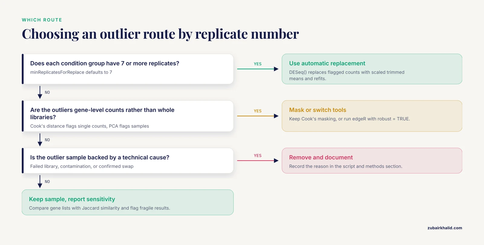
First, when you call DESeq() with the default minReplicatesForReplace = 7, any condition group with at least 7 replicates gets automatic outlier replacement. Flagged counts are replaced by a trimmed mean (the default trims 0.2 from each tail) scaled by size factors, and the model is refit. Second, when a group has fewer than 7 replicates, nothing is replaced. Instead, results() applies a Cook's distance cutoff, the 0.99 quantile of the F distribution with p and m - p degrees of freedom (p is the number of model parameters, m is the number of samples), and sets the p-values of flagged genes to NA.
What edgeR does by default
edgeR never edits your counts. Its robustness lives in the dispersion estimation step. estimateDisp(y, design, robust = TRUE) and glmQLFit(y, design, robust = TRUE) turn on robust empirical Bayes squeezing, so genes with outlying dispersions contribute less to the trend that every other gene borrows from. Both default to robust = FALSE, which is the most common reason edgeR runs behave worse than expected on messy data. The quasi-likelihood (QL) pipeline, glmQLFit followed by glmQLFTest, adds a second layer of variance shrinkage that keeps error rates controlled at small sample sizes, which is why the edgeR documentation recommends it over the likelihood ratio test for standard group comparisons.
What benchmarks say about tool choice
Method comparisons disagree more than most analysts expect. A benchmark using RNA spike-in data (synthetic transcripts added at known concentrations) and simulations found that DESeq2, a robust variant of edgeR, and voom (limma's mean-variance weighted method) with TMM normalization or sample weights performed well overall regardless of outlier presence and the proportion of differentially expressed genes, while also showing that results depend heavily on which benchmark you trust [3].
A comparison of edgeR and DESeq2 on real and semi-simulated bulk data, mostly from human patients, found that DESeq2 generally identified more differentially expressed genes at smaller sample sizes, that the two tools became more concordant as sample size grew, and that both responded similarly to simulated outliers, with the Jaccard similarity of their gene sets (the overlap between two sets divided by their union) falling as more swapped samples were introduced. The same study found edgeR delivered higher F1 scores (a combined precision and recall metric) in 9 of 13 contrasts, using Bonferroni-adjusted p < 0.05 (a conservative multiple testing adjustment) and |log2FC| > 1 as the significance criteria [4].
An updated six-dimensional comparison of 12 methods across 80 simulated and real datasets, scoring detection accuracy, sensitivity at low false discovery rate (FDR, the expected share of false positives among genes you call significant), false positives, stability, robustness to outliers, and robustness to noise, found no single winner. ABSSeq led at n = 3, DESeq2 and the edgeR quasi-likelihood framework (slightly ahead of the likelihood ratio test) gained sensitivity at n = 5 under stringent false positive control, DESeq produced fewer false positives than DESeq2 at a sensitivity cost, and Wilcoxon and ROTS were the robust choices for small samples [5].
Beyond the two big tools
DeClUt takes a different route entirely, clustering expression profiles and assigning samples to conditions so that results are robust to the outliers typical of RNA-seq data, with a lower false positive ratio than edgeR, DESeq2, NOISeq, and SAMseq in published tests [6]. aFold models count uncertainty with a polynomial across treatments and genes and uses qtotal normalization, which keeps fold changes comparable across experiments [2]. Both are worth knowing when your dataset violates NB assumptions outright.
Step-by-Step Robust Workflow for DESeq2 and edgeR Outliers
Run the steps in order and keep every intermediate object, because the verification step compares them.
Step 1: Install and load the packages
if (!requireNamespace("BiocManager", quietly = TRUE)) {
  install.packages("BiocManager")
}
BiocManager::install(c("DESeq2", "edgeR"))

library(DESeq2)
library(edgeR)
Step 2: Import counts and metadata, then filter
DESeq2 requires non-negative integer counts. If your counter produced integers (featureCounts, HTSeq), a round() guard is harmless. Row names of the sample table must match column names of the count matrix exactly.
cts <- as.matrix(read.csv("counts.csv", row.names = 1))
coldata <- read.csv("metadata.csv", row.names = 1)
coldata$condition <- factor(coldata$condition, levels = c("control", "treated"))

stopifnot(identical(colnames(cts), rownames(coldata)))

dds <- DESeqDataSetFromMatrix(countData = round(cts),
                              colData  = coldata,
                              design   = ~ condition)

# Keep genes with at least 10 reads in at least 5 samples
keep <- rowSums(counts(dds) >= 10) >= 5
dds <- dds[keep, ]
table(keep)
Expected output:
FALSE  TRUE
 3211 15234
Filtering matters for outlier handling, not just speed. Genes with near-zero counts produce unstable dispersion estimates that look exactly like outliers and pollute the trend that well-behaved genes borrow from.
Step 3: Detect sample-level outliers before any model
vsd <- vst(dds, blind = FALSE)   # variance stabilizing transform for visualization
plotPCA(vsd, intgroup = "condition")

round(colSums(counts(dds)) / 1e6, 1)   # library size in millions of reads
The PCA should show control and treated separating along the first principal component, with replicates clustering inside their group. A sample sitting far from its group, or a library size several-fold below the others, is a candidate sample-level outlier. The blind = FALSE argument tells the transform to use the design, which is correct once you have verified the design.
Decision rule: remove a sample only with a documented technical cause, such as a failed library, contamination, or a confirmed swap, and record the reason in your script and your methods section. If the cause is unknown, keep the sample and use the robust options in the next steps.
Step 4: Run DESeq2 with automatic outlier replacement
dds <- DESeq(dds, minReplicatesForReplace = 7)
res <- results(dds, alpha = 0.05)
summary(res)
Expected console output from DESeq():
estimating size factors
estimating dispersions
gene-wise dispersion estimates
mean-dispersion relationship
final dispersion estimates
fitting model and testing
If any group has at least 7 replicates and contains flagged outliers, DESeq2 prints an additional message that it is replacing outliers and refitting, along with the number of genes affected. With 10 samples per group, replacement is active.
Expected output from summary(res):
out of 15234 with nonzero total read count
adjusted p-value < 0.05
LFC > 0 (up)       : 612, 4%
LFC < 0 (down)     : 548, 3.6%
outliers [1]       : 0, 0%
low counts [3]     : 4310, 28%
(mean count < 8)
[1] see 'cooksCutoff' argument of ?results
[3] see 'independentFiltering' argument of ?results
The outliers line counts genes masked by Cook's filtering. After successful replacement it should be 0. The alpha argument sets the target FDR for independent filtering, DESeq2's removal of low-mean genes before multiple testing adjustment, and defaults to 0.1. Setting 0.05 aligns filtering with the threshold you will actually use.
Inspect gene-level outliers directly:
boxplot(log10(assays(dds)[["cooks"]]), range = 0, las = 2)
plotDispEsts(dds)
In the Cook's boxplot, samples with many genes far above the pack deserve a second look. In the dispersion plot, the shrunken values should sit near the trend, with a cloud of raw estimates around it. A wall of raw dispersions far above the trend means either real biological heterogeneity or unhandled outliers.
Step 5: Handle the small-sample case explicitly
If your groups have fewer than 7 replicates, for example 3 versus 3, replacement never activates and Cook's masking takes over. Build the object the same way and run:
dds_small <- DESeq(dds_small)
res_small    <- results(dds_small)
res_small_nc <- results(dds_small, cooksCutoff = FALSE)

sum(is.na(res_small$padj))
sum(is.na(res_small_nc$padj))
Expected output:
[1] 1204
[1] 962
The drop between the two numbers is the set of genes that Cook's masking had removed. With cooksCutoff = FALSE those genes become testable again, but you have chosen to keep the outlier's influence on them, so say so in your methods. The remaining NAs come from independent filtering and mean low counts, not outliers. A useful middle path at small n is to keep the default masking and cross-check the flagged genes with a model-free Wilcoxon rank-sum test on the raw counts, which takes one line per gene and gives you a second opinion.
Step 6: Run edgeR with robust dispersion and quasi-likelihood fitting
y <- DGEList(counts = cts, group = coldata$condition)
design <- model.matrix(~ condition, data = coldata)

keep <- filterByExpr(y, design)
y <- y[keep, , keep.lib.sizes = FALSE]
y <- calcNormFactors(y)            # TMM normalization, trimmed mean of M values

y    <- estimateDisp(y, design, robust = TRUE)
fit  <- glmQLFit(y, design, robust = TRUE)
qlf  <- glmQLFTest(fit, coef = "conditiontreated")
topTags(qlf, n = 5)
Expected output:
Coefficient:  conditiontreated
            logFC logCPM      F   PValue      FDR
ENSG000001   2.41   6.12  96.31  1.4e-15  2.6e-11
ENSG000002   1.87   5.44  71.80  8.9e-14  8.3e-10
ENSG000003  -1.62   7.03  64.52  4.2e-13  2.6e-09
ENSG000004   3.05   4.88  58.14  1.7e-12  7.9e-09
ENSG000005  -2.20   5.01  52.73  5.5e-12  2.0e-08
Parameters that matter here:
robust = TRUEinestimateDisp()applies robust empirical Bayes squeezing of gene-wise dispersions toward the trend. Without it, a handful of dispersion-outlier genes can drag the trend upward and cost power across the whole table.robust = TRUEinglmQLFit()does the same for the quasi-likelihood dispersion, the second variance layer that drives the F-test.coefselects the design column to test. For arbitrary comparisons, such as interaction terms, pass acontrastvector built withmakeContrasts()instead.keep.lib.sizes = FALSErecomputes library sizes after filtering, which keeps TMM scaling honest.
Check the fit with the two standard diagnostics:
plotBCV(y)      # biological coefficient of variation, trend plus common estimate
plotQLDisp(fit) # QL dispersion before and after squeezing
You want the squeezed QL dispersion points hugging the trend, with a modest spread. A funnel shape or a cluster of points far above the trend line points to genes whose variance the model does not trust, which is exactly where robust fitting earns its keep.
Step 7: Add winsorization for large population-style datasets
Winsorization caps each gene's counts at a chosen quantile, so a single runaway sample cannot dominate that gene's dispersion. The published evaluation behind this approach was carried out on human population-scale datasets, so treat it as a large-sample tool rather than a default for small experiments [1]. A generic implementation looks like this:
winsorize_by_group <- function(counts, group, p) {
  out <- counts
  for (g in unique(group)) {
    idx  <- which(group == g)
    mat  <- counts[, idx, drop = FALSE]
    caps <- apply(mat, 1, quantile, probs = p)
    out[, idx] <- pmin(mat, caps)
  }
  dimnames(out) <- dimnames(counts)
  round(out)
}

cts_win <- winsorize_by_group(cts, coldata$condition, p = 0.95)

dds_win <- DESeqDataSetFromMatrix(countData = cts_win,
                                  colData  = coldata,
                                  design   = ~ condition)
dds_win <- dds_win[rowSums(counts(dds_win) >= 10) >= 5, ]
dds_win <- DESeq(dds_win)
res_win <- results(dds_win, alpha = 0.05)
Three practical points. The quantile p is a real parameter, not decoration, and the evaluated settings are described in the source publication, so match them rather than guessing. Winsorization lowers counts, so re-run your filtering and let normalization re-estimate from scratch, as the code above does. And capping changes the log2 fold change of the capped sample, which is the price of protecting the dispersion estimate. With only 3 samples per group, a 95th percentile cap barely bites, which is one more reason the method belongs to large studies.
Step 8: Verify, compare, and document
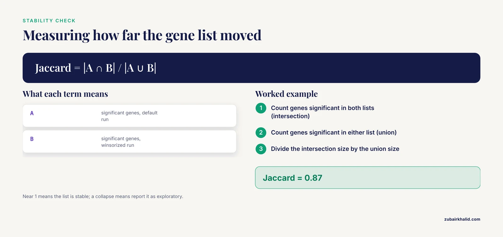
The single most informative check is a sensitivity analysis: rerun the analysis with and without the outlier handling and measure how much the significant set moves. Jaccard similarity, the size of the intersection divided by the size of the union, is the standard way to express that movement in method comparisons [4].
sig_default <- rownames(subset(res,      padj < 0.05))
sig_win     <- rownames(subset(res_win,  padj < 0.05))

jaccard <- length(intersect(sig_default, sig_win)) /
           length(union(sig_default, sig_win))
jaccard
Expected output:
[1] 0.87A value near 1 means the gene list is stable under your outlier choices. A value that collapses when you change one setting means the list is fragile and should be reported as exploratory. Finish with the reproducibility record and sensible next steps:
sessionInfo()Report software versions, keep both gene lists in supplementary files, and consider lfcShrink() in DESeq2 or glmTreat() in edgeR when you want fold-change thresholds to carry uncertainty estimates rather than raw maximum likelihood values.
Outlier-Handling Options at a Glance
| Situation | Command | What it does | Caveat |
|---|---|---|---|
| Gene-level outlier, 7 or more replicates per group | DESeq(dds, minReplicatesForReplace = 7) | Replaces flagged counts with size-factor scaled trimmed means and refits | Silent at smaller group sizes |
| Gene-level outlier, fewer than 7 replicates | results(dds, cooksCutoff = FALSE) | Stops p-value masking so flagged genes stay testable | You keep the outlier's influence, so report it |
| Dispersion outliers across genes | estimateDisp(y, design, robust = TRUE) | Robust empirical Bayes squeezing toward the trend | Not the default, must be requested |
| QL dispersion outliers | glmQLFit(y, design, robust = TRUE) | Robust squeezing of the quasi-likelihood dispersion | Pair with glmQLFTest() |
| Sample-level outlier | vst() plus plotPCA() or plotMDS() | Detection and documentation | Removal needs a technical cause |
| Many samples per condition, population-scale data | Winsorize counts, then rerun DESeq2 or edgeR | Caps extreme counts so one sample cannot dominate a gene's dispersion | Evidence base is large datasets, refilter and renormalize after |
| Small groups, exploratory analysis | Wilcoxon rank-sum or ROTS as cross-checks | Model-free or robust second opinion | Lower sensitivity to effect size |
Bioinformatics Troubleshooting: Exact Errors and Fixes
The model matrix is not full rank
Error in checkFullRank(modelMatrix) :
  the model matrix is not full rank, so the model cannot be fit as specified.
  One or more variables or interaction terms in the design formula are linear
  combinations of the others and must be removed
Cause: a design column is redundant, for example ~ batch + condition + batch_condition_combo where the combo encodes the other two, or an interaction without main effects in a balanced design. Fix by dropping the redundant term. Verify with qr(model.matrix(~ condition + batch, coldata))$rank == ncol(model.matrix(~ condition + batch, coldata)). edgeR fails the same way on rank-deficient designs inside glmFit, with the same remedy.
Every gene contains at least one zero
Error in estimateSizeFactorsForMatrix(counts(object)) :
  every gene contains at least one zero, cannot compute log geometric means
Cause: DESeq2's median-of-ratios size factor estimator needs a geometric mean per gene, and any zero in a gene's row makes that mean zero. This happens with very sparse or very deep datasets. Fix with dds <- estimateSizeFactors(dds, type = "poscounts"), or filter genes that are zero in many samples before building the object.
Duplicate row names on import
Error in `.rowNamesDF<-`(x, value = value) : duplicate 'row.names' are not allowedCause: gene symbols map to multiple loci, so your count table has repeated identifiers. Fix by aggregating counts per symbol (sum them) before import, or work with stable Ensembl gene IDs and map to symbols only for reporting.
A wall of NA adjusted p-values
Not an error message, a behavior. Two documented mechanisms set padj to NA: Cook's distance masking at small replicate numbers, and independent filtering of low-mean genes. Diagnose with sum(is.na(res$padj)) before and after results(dds, cooksCutoff = FALSE), and inspect mcols(dds)$maxCooks for the flagged genes. Treat NA as untested in downstream code, never as zero and never as significant.
Calling the test before the fit in edgeR
If you run glmQLFTest() on a DGEList that never passed through glmQLFit(), edgeR stops with an error saying no fitted model was found. The fix is procedural: estimateDisp(), then glmQLFit(), then glmQLFTest(), in that order, every time.
Common Mistakes and Limitations
- Deleting samples without a documented technical cause. Sample removal is a judgment call that can bias human studies. Detect with PCA and depth metrics, justify in writing, and report a sensitivity analysis with the sample included.
- Assuming replacement runs automatically at n = 3. The default
minReplicatesForReplace = 7means small groups never get replacement. Many analysts believe DESeq2 "handled" their outliers when the mechanism never fired. - Setting
cooksCutoff = FALSEto make NAs disappear. This is a legitimate choice, but it re-admits every influential observation. Report it, and cross-check the affected genes. - Confusing sample-level and gene-level outliers. PCA finds bad libraries, Cook's distance finds bad counts. Using one tool to hunt the other's target wastes an afternoon.
- Forgetting
robust = TRUEis not the default in edgeR. A plainestimateDisp()call gives you the non-robust trend. On messy datasets the robust version is the one the benchmarks evaluated favorably [3]. - Winsorizing small experiments. The supporting evidence comes from large human population datasets [1]. At 3 samples per group a high quantile cap barely changes anything while altering fold changes, so you take the distortion without the protection.
- Treating one benchmark result as universal. Performance depends on the benchmark, the proportion of DE genes, and sample size, and no single method wins across all criteria and scenarios [3][5]. Pick the tool that matches your n and your noise, then verify.
- Ignoring upstream causes. A sample swap, barcode bleed, or bad alignment will defeat any downstream robustness. Fix the data first, the model second.
- Reading NA
padjas zero or as significant. NA means untested. Scripts that subset withpadj < 0.05silently drop NA rows, which is usually what you want, but scripts that testis.na()incorrectly or impute zeros corrupt the result. - Filtering too hard or not at all. Unfiltered low-count genes destabilize the dispersion trend and masquerade as outliers, while over-filtering discards real low-abundance biology. The
rowSums(counts >= 10) >= 5andfilterByExpr()patterns above are sane starting points. - Not recording versions. DESeq2 and edgeR defaults have changed across releases.
sessionInfo()in the script directory is the cheapest insurance a reproducibility reviewer will ever ask of you.
A final limitation: most outlier evidence comes from simulations and semi-simulated data, where outliers are planted on purpose. Real outliers arrive with causes you may never identify, so treat every robust method as damage control rather than a license to skip QC, and have a statistician sign off before any sample leaves a human dataset.
Frequently Asked Questions
Should I delete outlier samples before running DESeq2 or edgeR?
Only when you have a documented technical cause such as a failed library, contamination, or a confirmed sample swap. Otherwise keep the sample, use the robust options described above, and report a sensitivity analysis showing how the gene list changes.
What does minReplicatesForReplace do in DESeq2?
It sets the minimum number of replicates a group needs before DESeq2 will automatically replace gene-level outlier counts and refit the model. The default is 7, so with fewer replicates nothing is replaced and Cook's distance masking in results() takes over instead.
Why are so many p-values NA in my DESeq2 results?
Two documented mechanisms set adjusted p-values to NA: Cook's distance masking when a gene has an influential observation, and independent filtering of low-count genes. NA means the gene was not tested, not that it failed to reach significance.
Does edgeR have an equivalent of DESeq2's replaceOutliers?
No, edgeR never edits your counts. Its robustness comes from robust empirical Bayes squeezing, which you enable with robust = TRUE in estimateDisp() and glmQLFit().
When should I winsorize counts before differential expression analysis?
The published evidence supports winsorization mainly for large population-scale datasets with many samples per condition. For a small two-condition experiment it has little effect and alters fold changes, so treat it as an option to test rather than a default.
How many replicates do I need for outlier-robust differential expression?
More replicates help every robust method, and automatic outlier replacement in DESeq2 needs a minimum per group before it activates. With very small groups, treat results as exploratory and consider a rank-based method as a cross-check.
Should I use glmQLFTest or glmLRT in edgeR?
Use glmQLFTest() for standard group comparisons, because the quasi-likelihood F-test controls small-sample error rates better. Keep glmLRT() for tests that QLF cannot express, such as comparing whole model fits with and without a term.
How do I check whether an outlier actually changed my results?
Run the analysis twice, once with and once without the outlier handling, then compute the Jaccard similarity of the two significant gene sets and inspect the Cook's distance boxplots. A large drop in similarity tells you the gene list is unstable and should be reported as such.
Sources
- Winsorization greatly reduces false positives by popular differential expression methods when analyzing human population samples.
- aFold - using polynomial uncertainty modelling for differential gene expression estimation from RNA sequencing data.
- Benchmarking RNA-seq differential expression analysis methods using spike-in and simulation data.
- Tool choice matters: Evaluating edgeR vs. DESeq2 for sensitivity, robustness, and cross-study performance.
- Revisiting differential expression analysis: An updated six-dimensional comparative study.
- DeClUt: Decluttering differentially expressed genes through clustering of their expression profiles.