Cross-Platform Normalization for RNA-seq and Microarray
By Dr. Zubair Khalid, DVM, MS, PhD ·

By the end of this guide you will be able to take one microarray matrix and one RNA-seq matrix, map both onto a shared gene identifier space, normalize each platform correctly on its own, apply a cross-platform normalization method such as quantile normalization, Training Distribution Matching (TDM), z-score standardization, or ComBat, and validate that the merged matrix behaves like a single coherent dataset. You will also know which normalization to pick for machine learning, differential expression, and clustering, and how to diagnose the failures that make integrated datasets fall apart silently.
You need R 4.3 or newer, Bioconductor, and these packages installed before you start:
install.packages("BiocManager")
BiocManager::install(c(
  "limma", "DESeq2", "sva", "oligo", "tdm",
  "hgu133plus2.db", "AnnotationDbi", "ggplot2"
))
The tdm package implements Training Distribution Matching and is distributed by the authors of the original TDM study [1]. If your microarray data come as raw CEL files you also want oligo or affy. If you only have processed matrices from GEO, which is the most common situation, you can skip the raw-file steps.
Everything here assumes two data frames, array_mat and seq_mat, with genes as rows and samples as columns.
Why RNA-seq and Microarray Data Disagree
The two platforms measure the same biology through different physics. A microarray reports hybridization intensity per probe, with a compressed dynamic range and a nonzero background floor. RNA-seq reports read counts per gene, with a wide dynamic range, many exact zeros, and count-based noise that grows with abundance. A direct merge of a log2 intensity matrix and a raw count matrix produces two blobs that separate perfectly by platform in a PCA plot, which is the classic sign that technical variance has overwhelmed biological signal.
Three specific technical differences recur across comparative studies. First, detection sensitivity differs at the low end. In a paired RNA-seq and microarray study of canine lymphoma, RNA-seq was more sensitive for detecting transcripts expressed at low levels, and RNA-seq sample variation tracked transcript GC content in a way microarray variation did not [2]. Second, probe coverage differs. A microarray probe set may cover a subset of a gene's transcripts, while RNA-seq counts all reads assigned to the gene, so isoform-level comparisons need explicit transcript abundance estimation and fold change normalization against a control rather than raw abundance comparison [3]. Third, the distributions have different shapes. Microarray log intensities look roughly symmetric and light tailed, while log RNA-seq counts are zero inflated and skewed, so a method that matches the marginal distribution of one platform to the other has to handle both shape and support differences [4].
The practical consequence is that no single transform fixes everything. Comparative evaluations have converged on a clear picture: you normalize within each platform first, then apply a cross-platform method, then choose downstream analyses that match the method's strengths and weaknesses [1][2][3].
Methods at a Glance
The evaluation of ten batch correction approaches for combined microarray and RNA-seq data grouped methods into three families: unsupervised sample-wise methods, unsupervised gene-wise methods, and supervised methods that use outcome labels during correction [5]. The table below summarizes the options you will actually encounter.
| Method | What it does | Family | Best suited for | Main caveat |
|---|---|---|---|---|
| Log2 transform (log2 CPM or log2 counts) | Compresses counts to a log scale | Sample-wise preprocessing | First step for RNA-seq before any merging | Does not align platform distributions by itself |
| Z-score per gene | Centers and scales each gene within a platform | Sample-wise / unsupervised | Pathway analysis, some ML tasks [4] | Standardization parameters must be computed per platform, never per batch |
| Quantile normalization | Forces identical marginal distributions across datasets | Unsupervised | Supervised and unsupervised ML on merged data [1][3] | Can remove predictive signal in some prediction tasks [6] |
| TDM (Training Distribution Matching) | Transforms RNA-seq data to match a microarray training distribution | Unsupervised | Applying a classifier trained on legacy arrays to RNA-seq [1] | Requires a reference training set, one directional |
| Nonparanormal transform | Gaussianizes data nonparametrically | Unsupervised | Pathway analysis with PLIER and related tools [4] | Less consistent for general ML than quantile or TDM |
| FSQN (feature-specific quantile normalization) | Quantile normalization applied per feature group | Unsupervised | Cross-platform subtype classification [7] | Needs enough RNA-seq samples to work well |
| ComBat / limma removeBatchEffect | Empirical Bayes gene-wise location and scale adjustment | Unsupervised gene-wise | Differential expression with proper Type I error control [5] | Needs a valid batch design, can overcorrect real biology |
| SVA | Decomposes variation into expression, platform, and latent factors | Unsupervised latent factor | Paired platform datasets, latent variation cleanup [2] | Surrogate variables can absorb biology if not protected |
| Rank-based methods (Rank-in, REO signatures) | Uses within-sample expression ordering rather than absolute values | Unsupervised | Signatures that transfer across platforms [13] | Discards magnitude information, works on relative order |
| PXN | Probabilistic translation between platform representations | Unsupervised learned model | Large-scale repository integration [8] | Requires training a model, newer tool with less field history |
Supervised correction methods sit at the most-processed end of the spectrum in the same evaluation. They achieved strong distribution alignment and clustering by biological group, but they leaked outcome information and inflated Type I error, which makes them unsuitable for unbiased discovery work [5].
Step-by-Step Cross-Platform Normalization Workflow
This section is the core walkthrough. Work through it in order, because each step depends on the previous one.
Step 1: Map Everything to a Shared Gene Identifier Space
Microarray platforms report probe IDs. RNA-seq pipelines report Ensembl IDs, gene symbols, or both. Before any normalization comparison can work, both matrices must have the same row identifiers, one row per gene, with the same gene set in the same order.
For an Affymetrix HG-U133 Plus 2.0 array, the common case in public data, map probes with the platform annotation package:
library(hgu133plus2.db)
library(AnnotationDbi)

probe_ids <- rownames(array_mat)
gene_map  <- AnnotationDbi::select(
  hgu133plus2.db,
  keys    = probe_ids,
  columns = c("SYMBOL"),
  keytype = "PROBEID"
)

# Collapse multiple probes per gene by the probe with highest mean intensity
gene_map <- gene_map[!is.na(gene_map$SYMBOL), ]
mean_by_probe <- rowMeans(array_mat, na.rm = TRUE)
gene_map$mean_expr <- mean_by_probe[gene_map$PROBEID]
gene_map <- gene_map[order(gene_map$mean_expr, decreasing = TRUE), ]
gene_map <- gene_map[!duplicated(gene_map$SYMBOL), ]

array_mat <- array_mat[gene_map$PROBEID, ]
rownames(array_mat) <- gene_map$SYMBOL
Expected result for a GPL570-style matrix:
dim(array_mat)
# [4] 54675   120        before mapping
dim(array_mat)
# [4] 18997   120        after symbol mapping and deduplication
The exact collapsed row count depends on the platform and annotation build. The number you should never accept is anything close to the original probe count, because that means duplicate symbols survived.
Then intersect with the RNA-seq gene list:
common_genes <- intersect(rownames(array_mat), rownames(seq_mat))
array_mat <- array_mat[common_genes, ]
seq_mat   <- seq_mat[common_genes, ]
Write the intersection size down. Tens of thousands of shared genes is normal for a whole-transcriptome human array. A few thousand suggests the two annotation builds disagree and you should re-map one side before continuing.
Step 2: Normalize Within Each Platform First
Cross-platform methods assume each input is already reasonably normalized on its own. This is where a common RNA seq error begins, when analysts feed raw counts or raw intensities into a batch correction step and the correction then has to absorb within-platform nuisance variation plus platform differences at the same time.
For microarray, use RMA on raw CEL files, or use limma's between-array normalization if you only have processed values. The Vibrio cholerae cross-platform integration study combined Rank-in with limma's normalizeBetweenArrays on the array side [9]:
library(limma)

# Raw CEL files
library(oligo)
raw <- read.celfiles(list.files("cel_dir/", full.names = TRUE))
array_norm <- rma(raw)
array_mat  <- exprs(array_norm)

# Processed matrix fallback
array_mat <- normalizeBetweenArrays(array_mat, method = "quantile")
normalizeBetweenArrays with method = "quantile" equalizes the intensity distributions across arrays. For processed GEO data already log2 transformed and quantile normalized, verify that before re-normalizing, because double normalization is a frequent and silent mistake.
For RNA-seq, compute size factors, then apply a variance-stabilizing transformation. The Arabidopsis stress integration study used variance-stabilizing transformation for RNA-seq normalization before cross-platform harmonization [10]:
library(DESeq2)

dds <- DESeqDataSetFromMatrix(
  countData = round(seq_mat),
  colData   = seq_coldata,
  design    = ~ 1
)

# Remove genes with near-zero counts before size factor estimation
keep <- rowSums(counts(dds) >= 10) >= 3
dds  <- dds[keep, ]
dds  <- estimateSizeFactors(dds)
seq_vst <- assay(vst(dds))
The gene filter step is not cosmetic. Without it you get the error covered in the troubleshooting section, and even when size factor estimation succeeds, thousands of all-zero rows add pure noise to every downstream distribution match.
Step 3: Put Both Matrices on a Comparable Scale
After Step 2, your array matrix is log2 scale. Your RNA-seq matrix from vst() is on a log-like scale but not identical in range. Two options work here, and the choice depends on the downstream task.
Option A, a plain log2 transform on normalized counts:
lib_sizes <- colSums(counts(dds))
seq_log   <- log2(t(t(counts(dds)) / lib_sizes) * 1e6 + 1)
Option B, keep the vst() output. The variance-stabilizing route preserved consensus differential expression signals in the plant integration study [10] and avoids the count-dependent mean variance trend that plain log2 of raw normalized counts still carries.
At this point both matrices have genes as rows in identical order. Confirm it explicitly, because a mismatch here produces the most dangerous failure mode in the entire workflow, a silent merge of misaligned rows:
identical(rownames(array_mat), rownames(seq_mat))
# [4] TRUE
If this returns FALSE, stop and fix it. Nothing downstream can be trusted from a misaligned merge.
Step 4: Apply the Cross-Platform Normalization
This is the step the whole article is named for. Here are the three most defensible default choices with working code.
Quantile normalization across the merged matrix. Quantile normalization forces both platforms to share one empirical distribution. Supervised and unsupervised machine learning evaluations found it, along with TDM, suitable for training models on microarray and RNA-seq data simultaneously [4]:
merged <- cbind(array_mat, seq_vst)
merged_q <- normalizeBetweenArrays(merged, method = "quantile")

# Split back apart if needed for validation
array_q <- merged_q[, colnames(array_mat)]
seq_q   <- merged_q[, colnames(seq_vst)]
Quantile normalization is aggressive. Every sample ends up with the same value distribution, which is exactly what you want when platform artifacts drive the distributions, and exactly what you do not want when genuine distributional differences between conditions carry predictive signal. A drug response modeling study found that z-score and log2 normalization substantially outperformed quantile normalization at preserving predictive signal across platforms, reaching a mean cross-validation AUC of 0.824 and an external RNA-seq test AUC of 0.821 [6].
Z-score standardization per gene, per platform. Compute the mean and standard deviation of each gene within each platform, then merge the standardized values:
zscore_cols <- function(m) {
  mu <- rowMeans(m, na.rm = TRUE)
  sd <- apply(m, 1, sd, na.rm = TRUE)
  t((t(m) - mu) / sd)
}

array_z <- zscore_cols(array_mat)
seq_z   <- zscore_cols(seq_vst)
merged_z <- cbind(array_z, seq_z)
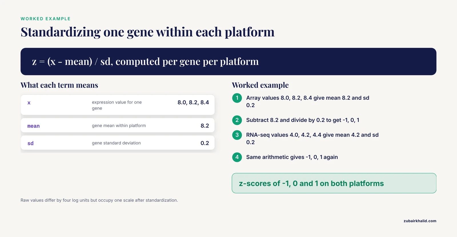
A tiny worked example makes the arithmetic concrete. Suppose gene X has log2 expression values of 8.0, 8.2, 8.4 across three arrays, mean 8.2 and standard deviation 0.2. The z-scores are -1, 0, and 1. The same gene reads 4.0, 4.2, 4.4 in vst-transformed RNA-seq, mean 4.2, standard deviation 0.2, giving z-scores of -1, 0, and 1 again. After standardization the gene occupies the same scale in both matrices even though its raw values differ by four log units.
Z-scores are explicitly appropriate for some applications, including pathway analysis with the Pathway-Level Information Extractor (PLIER), in the systematic ML evaluation [4]. Keep in mind what they discard: absolute abundance. A gene expressed at moderate levels in one platform and high levels in another can look identical after standardization.
Training Distribution Matching. TDM was developed specifically to transform RNA-seq data for use with models trained on legacy microarray platforms, and it showed consistently strong performance across supervised and unsupervised evaluation settings, outperforming quantile normalization, a nonparanormal transform, and plain log2 in many circumstances [1]:
library(tdm)
# ?tdm_adjust documents the version-specific arguments.
# TDM learns a mapping from the RNA-seq distribution
# toward the array training distribution, so the array
# matrix stays untouched and only the RNA-seq side moves.
TDM is one-directional by design. The array data are the reference, the RNA-seq data are adjusted toward them. Use it when the situation is exactly that, a trained model or established array-based reference that must accept RNA-seq input. If both platforms are equal partners in an exploratory integration, symmetric methods such as quantile normalization or ComBat fit better.
ComBat as the gene-wise option. When the downstream goal is differential expression or when you want batch correction with documented error control properties, apply ComBat after within-platform normalization and a log2-like transform:
library(sva)

batch <- c(rep("array", ncol(array_mat)), rep("rnaseq", ncol(seq_vst)))
mod   <- model.matrix(~ 1, data = data.frame(batch = batch))

merged_combat <- ComBat(
  dat   = cbind(array_mat, seq_vst),
  batch = batch,
  mod   = mod
)
Gene-wise empirical Bayes methods like this maintained appropriate Type I error control and achieved higher power in the differential expression evaluation, with limma showing the strongest DE performance among tested methods [5]. Note that limma's removeBatchEffect serves the same purpose for visualization and modeling contexts, and the ComBat call above should never include your outcome of interest in mod for discovery work, for reasons covered under Common Mistakes.
Step 5: Validate the Integrated Matrix
Never ship a merged matrix without three checks.
First, PCA before and after. The merged matrix should show platform separation before cross-platform normalization and mixed samples afterward:
library(ggplot2)

pca_plot <- function(m, title) {
  pcs <- prcomp(t(m), center = TRUE, scale. = FALSE)
  df  <- data.frame(
    PC1 = pcs$x[, 1], PC2 = pcs$x[, 2],
    platform = c(rep("array", ncol(array_mat)),
                 rep("rnaseq", ncol(seq_vst)))
  )
  ggplot(df, aes(PC1, PC2, color = platform)) +
    geom_point(size = 2) +
    ggtitle(title)
}

pca_plot(cbind(array_mat, seq_vst),   "Before cross-platform normalization")
pca_plot(merged_combat,               "After ComBat")
Expected output: in the first plot, PC1 or PC2 separates the two platform colors cleanly. After a successful normalization, the colors interleave. If platform colors still separate after correction, the method failed or the gene intersection is too small.
Second, correlation on paired samples if you have them. AnyExpress reported mean within-platform Pearson correlation of 0.98 for its kidney and liver case study data as a benchmark of what well-behaved expression matrices look like [11]. For paired microarray and RNA-seq samples on the same biological specimens, gene-level Pearson correlation after normalization should land well above 0.8 in well-behaved datasets. Values near 0.5 signal a mapping or normalization problem, not subtle biology.
Third, for clustering work, verify that subtypes recovered from the merged matrix agree with subtypes recovered from each platform alone. The lung cancer study tested 384 combinations of data processing methods across more than 3500 lung samples and evaluated that agreement explicitly, which is the right template for your own validation [12].
Step 6: Route to the Right Downstream Analysis
The normalization choice and the analysis choice are coupled. Here is the mapping the literature supports.
Machine learning classification. Quantile normalization and TDM are the two methods validated for training on merged microarray and RNA-seq data across both supervised and unsupervised settings [1][3]. Feature-specific quantile normalization reached up to 98 percent accuracy for breast invasive carcinoma and 97 percent for colorectal cancer molecular subtype classification, using support vector machines trained exclusively on microarray data and applied to FSQN-normalized RNA-seq [7]. Independent training and testing on TCGA breast cancer data also showed that selecting non-differentially expressed genes for normalization and differentially expressed genes for classification improved cross-platform model performance, and that nonparametric normalization outperformed parametric approaches [13].
Differential expression. Do not DE-test a merged, batch-corrected matrix as if it were one experiment. The robust pattern is to run differential expression within each platform, DESeq2 for RNA-seq and limma for microarray, then combine. That is the structure used in the liver fibrosis integration, which ran DESeq2 on RNA-seq and limma on microarray within each dataset before harmonizing gene-level matrices with ComBat for downstream network and ordination analyses [14]. The comparative evaluation supports this design, because gene-wise unsupervised correction preserved Type I error while supervised correction inflated it, and meta-analysis combining p-values across platforms was also effective [5].
Clustering and subtype discovery. Unsupervised learning on combined data is achievable with careful preprocessing and cross-platform normalization, as demonstrated across the 384-combination lung cancer evaluation [12]. Quantile-based and TDM-based normalization both supported unsupervised model training in the broader ML assessment [4].
Signatures that must survive platform transfer. If your real goal is a compact biomarker panel that works on both platforms, consider rank-based approaches that discard absolute values entirely. A within-sample relative expression ordering (REO) signature of nine gene pairs reached 97.53 percent accuracy in five-fold cross-validation for early pancreatic ductal adenocarcinoma and validated successfully on both microarray and RNA-seq data [15]. A mucoepidermoid carcinoma signature built on two microarray cohorts transferred with good reproducibility to an independent RNA-seq cohort [16].
Common Mistakes and Limitations
These are the failures that show up repeatedly in real cross-platform projects.
- Normalizing before collapsing probes. If three probes map to one gene and you average them after cross-platform normalization instead of before, the averaging happens in the wrong space and the gene's distribution is a blend that no longer matches either platform. Collapse probe sets first, always.
- Using supervised batch correction for discovery. Supervised methods achieved the best apparent alignment in the ten-method evaluation, but they leaked outcome information and inflated Type I error, which makes any subsequent differential expression or biomarker claim unreliable [5]. Reserve them for prediction pipelines where the outcome is known for every sample by design and you accept the leakage framing.
- Trusting high AUROC across a platform transfer. High AUROC measures rank discrimination, not whether a fixed decision threshold survives. In a sepsis classifier evaluation, training-derived standard and robust scaling produced balanced accuracy of 0.50 at the 0.5 threshold on the cross-platform RNA-seq cohort GSE154918 despite very high AUROC, meaning the classifier performed at chance at its operational threshold. A sample-wise rank strategy that avoided training-derived external scaling preserved balanced accuracy between 0.95 and 1.00 across external cohorts [17]. If a model will be deployed with a fixed cutoff, validate the cutoff, not just the curve.
- Applying quantile normalization when the task needs absolute signal. Quantile normalization destroys between-sample distribution differences, and when those differences carry the phenotype signal, predictive performance collapses. The drug response modeling comparison documented exactly this, with z-score and log2 normalization substantially outperforming quantile normalization for that prediction task [6]. Match the method to the task, not to habit.
- Underpowered RNA-seq side. FSQN achieved its best cross-platform subtype accuracy when normalizing RNA-seq datasets containing at least 25 samples [7]. With fewer RNA-seq samples, quantile-style methods estimate unstable target distributions. Plan sample numbers accordingly or switch to a method that leans on the array side as the reference, such as TDM.
- Feeding raw counts into cross-platform correction. This is the most common RNA seq error in integration projects. ComBat, quantile normalization, and z-scoring all assume roughly continuous, variance-stabilized inputs. Raw counts violate that on the RNA-seq side, so the correction spends its capacity absorbing count noise instead of platform effects. Normalize within platform first, every time.
- Silent gene misalignment. No error message announces that
gene BRCA1in your array matrix is row 500 while in your RNA-seq matrix it is row 1,832. Theidentical(rownames(...))check in Step 3 is the only cheap defense. Run it after every operation that touches row order.
- Expecting isoform-level agreement by default. Gene-level correlations between platforms are strong, but isoform-level comparisons require explicit transcript abundance estimation, and studies found fold change estimates against a control agree better across platforms and with RT-qPCR than raw abundance estimates do [3]. If your question lives below the gene level, budget for transcript-level pipelines such as those evaluated with eXpress, MMBGX, and RSEM [3].
- Letting surrogate variables eat biology. SVA decomposed paired lymphoma data cleanly into transcript abundance, technology, and latent variation components [2], but unmanaged surrogate variables can absorb real biological contrasts, particularly with unbalanced group sizes. Protect your design variables in the SVA model when group structure matters.
- Interpreting platform differences as biology. A gene that appears RNA-seq specific may simply lack a probe, and a gene that appears microarray specific may have cross-hybridizing probes. Detection sensitivity differences at low expression are a known platform property, documented in the paired lymphoma comparison where RNA-seq detected low-level transcripts the array missed [2]. Cross-check claims about platform-specific expression against annotation before writing them up.
Troubleshooting Guide
These are the concrete errors you will hit, with fixes.
"Error in estimateSizeFactorsForMatrix(counts(object), ...): every gene contains at least one zero, cannot compute log geometric means." This is the classic DESeq2 failure on sparse matrices. DESeq2's default size factor method needs genes with nonzero counts across all samples. Fix it by filtering before estimating size factors:
keep <- rowSums(counts(dds) >= 10) >= 3
dds  <- dds[keep, ]
dds  <- estimateSizeFactors(dds)
"Error in quantile.default(x, probs, na.rm = FALSE): missing values and NaN's not allowed." Quantile normalization cannot run on matrices containing NA values, which happen after probe-to-gene mapping when some probes lack annotation. Fix by removing genes with missing values, or by imputing only if your downstream method requires it:
merged <- na.omit(merged)Verify the remaining gene count is still large enough for meaningful integration. Losing a few thousand genes is normal, losing half your matrix means the annotation mapping needs rework.
"Error in ComBat(dat = ..., batch = ...): The number of columns of dat must equal the length of batch." Your batch vector does not match the merged column order. This almost always happens when you cbind the matrices in one order and build the batch vector from a metadata table sorted differently. Rebuild the vector from the actual column names:
batch <- ifelse(colnames(merged) %in% colnames(array_mat), "array", "rnaseq")"Error: cannot allocate vector of size 3.2 Gb." Merged whole-transcriptome matrices with tens of thousands of genes and hundreds of samples overflow memory during quantile normalization or PCA. Fix by running on a machine with more RAM, converting the matrix to a matrix of type numeric explicitly rather than keeping data frame overhead, or subsampling genes to the set that matters for your analysis.
PCA still shows two perfect platform clusters after ComBat. No error message here, which is what makes it dangerous. Diagnose in this order: check identical(rownames(...)), check that the RNA-seq side was log-transformed or vst-transformed before ComBat, check that the gene intersection contains more than a few thousand genes, and check that the batch assignment vector matched the columns correctly. In most failed integrations the root cause is one of those four.
Array-side values are on a 0 to 100 scale, not log2 scale. Some GEO series ship processed data as linear-scale or even signal counts. Quantile-normalizing a mix of log and linear data is meaningless. Detect this by looking at the value range and distribution:
summary(array_mat[, 1])
# Min. 0th Qu.  Median    Mean  3rd Qu.    Max.
#  5.1    6.8     7.9     8.3     9.2    14.1   # log2 scale, fine
# Min. 0th Qu.  Median    Mean  3rd Qu.    Max.
#  12     45      120     340     410     9800  # linear scale, must log2 transform
When in doubt, log2 transform the array side, since RMA output is already log2 and quantile normalization on log2 data is the standard state for these pipelines.
Everything looks fine but cross-platform predictions fail. Revisit mistake 3. If internal cross-validation AUC is high and external platform-transfer performance collapses at a fixed threshold, switch to a rank-based or strictly inductive preprocessing strategy rather than tuning the classifier further [17].
Sensible Next Steps
Once the basic pipeline runs, three directions extend it. For large-scale repository integration across many technologies, PXN provides a trained probabilistic translation between platforms, benchmarked above existing normalization methods for cross-platform accuracy and differential expression power [8]. For network-level interpretation of integrated data, feeding the harmonized matrix into WGCNA recovered meaningful functional modules in the Vibrio cholerae integration and in the liver fibrosis study [13]. For a fast check of robustness, re-derive your key result using only rank-based information, such as relative expression orderings [15], and see whether it survives, because agreement between value-based and order-based results is one of the cheapest strong signals that your integration captured biology rather than platform artifacts.
One limitation applies to any integrated analysis. Results from a merged cohort describe the populations and platforms in the data, and any translational decision for an individual case belongs with the relevant domain expert and validated clinical tools.
Frequently Asked Questions
Can I merge RNA-seq and microarray expression matrices directly?
No. The two platforms produce different value distributions, dynamic ranges, and noise structures, so a direct merge separates samples by platform rather than biology. Normalize within each platform, then apply a cross-platform normalization method such as quantile normalization, TDM, z-scoring, or ComBat before merging.
Which cross-platform normalization method should I use for machine learning?
Quantile normalization and TDM are the methods validated for supervised and unsupervised machine learning on combined microarray and RNA-seq data. Z-scores also work for some applications such as pathway analysis. For prediction tasks where absolute signal matters, compare z-score and log2 approaches against quantile normalization empirically.
Should I run ComBat before or after within-platform normalization?
After. ComBat and similar gene-wise methods assume variance-stabilized input, so run RMA or quantile normalization on the array side and size factors plus vst or log2 CPM on the RNA-seq side first, then apply ComBat to the merged, transformed matrices.
Can I do differential expression on a merged cross-platform matrix?
Prefer running differential expression separately within each platform, using DESeq2 for RNA-seq and limma for microarray, then combining results through meta-analysis. Direct testing on merged batch-corrected data risks inflated false positives, particularly if any supervised correction touched the data.
What is Training Distribution Matching?
TDM is a normalization method that transforms RNA-seq data so its distribution matches a microarray training set, letting models built on legacy array platforms accept RNA-seq input. The array data serve as the fixed reference and only the RNA-seq side is adjusted.
Why does my PCA still show two clusters after normalization?
The usual causes are a gene row misalignment between matrices, RNA-seq values that were never log or vst transformed, a gene intersection too small to carry shared signal, or a batch vector that does not match the merged column order. Check those four in that order.
How many RNA-seq samples do I need for feature-specific quantile normalization?
FSQN reached its best subtype classification accuracy when the RNA-seq dataset contained at least 25 samples. Below that, quantile-style target distributions are estimated too unstably for reliable platform bias removal.
Are there normalization-free approaches that transfer across platforms?
Yes. Methods based on within-sample relative expression orderings use the rank order of gene pairs inside each sample rather than absolute values, which makes them naturally robust to platform differences. They have produced diagnostic signatures validated on both microarray and RNA-seq data.
Sources
- Cross-platform normalization of microarray and RNA-seq data for machine learning applications.
- Comparative RNA-Seq and microarray analysis of gene expression changes in B-cell lymphomas of Canis familiaris.
- Comparative evaluation of isoform-level gene expression estimation algorithms for RNA-seq and exon-array platforms.
- Cross-platform normalization enables machine learning model training on microarray and RNA-seq data simultaneously.
- Evaluating Cross-Platform Batch Correction Methods for Integrated Microarray and RNA-seq Data Analysis.
- UCResponNet-X: cross-platform multi-dataset gene expression for predictive modeling of drug response in ulcerative colitis.
- Feature specific quantile normalization enables cross-platform classification of molecular subtypes using gene expression data.
- PXN Unlocks the Power of Public Gene Expression Data Through Cross-Technology Integration.
- Cross-Platform Transcriptomic Data Integration, Profiling, and Mining in Vibrio cholerae.
- Integrative cross-platform transcriptomic analysis coupled with machine learning identifies candidate biomarkers of abiotic stress resilience in Arabidopsis thaliana.
- AnyExpress: integrated toolkit for analysis of cross-platform gene expression data using a fast interval matching algorithm.
- Identification of transcriptional subtypes in lung adenocarcinoma and squamous cell carcinoma through integrative analysis of microarray and RNA sequencing data.
- Normalization and Selecting Non-Differentially Expressed Genes Improve Machine Learning Modelling of Cross-Platform Transcriptomic Data.
- Integrative Transcriptomics Across Etiologies Reveals Common and Disease-Specific Fibrogenic Signatures in Liver Fibrosis.
- Early Diagnosis of Pancreatic Ductal Adenocarcinoma by Combining Relative Expression Orderings With Machine-Learning Method.
- A cross-platform validated biomarker signature for mucoepidermoid carcinoma identified by integrated WGCNA and machine learning.
- High AUROC can mask decision failure in sepsis transcriptomic classifiers: Preprocessing stability outweighs post hoc calibration across cohorts.