How to Perform Comparative Genomics Analysis in R
By Dr. Zubair Khalid, DVM, MS, PhD ·

By the end of this guide, you will be able to run a complete comparative genomics analysis workflow in R: load genome sequences, compute length and GC content statistics, build multiple sequence alignments, measure divergence with nucleotide diversity and Ka/Ks, analyze codon usage bias, visualize genome structure, construct phylogenetic trees, test functional enrichment of candidate genes, and assemble a pan-genome presence/absence matrix. You will also know how to check each intermediate result so that errors surface early rather than in a final figure.
To follow along, you need R (version 4.2 or newer is reasonable), the Bioconductor package manager, roughly 8 GB of RAM for small-to-medium genomes, and a set of genome sequences in FASTA or GenBank format. R for bioinformatics has become a standard choice because the language combines statistical rigor with package-based interoperability. A review of R and Bioconductor in genomics highlights the breadth of available tools, the modular nature of packages, enforced interoperability, and version control as the main advantages of this ecosystem [1]. This article functions as a practical Bioconductor tutorial for one specific use case, comparative genomics, and every code block runs as written if your input files are in place.
What a Comparative Genomics Analysis Workflow in R Includes
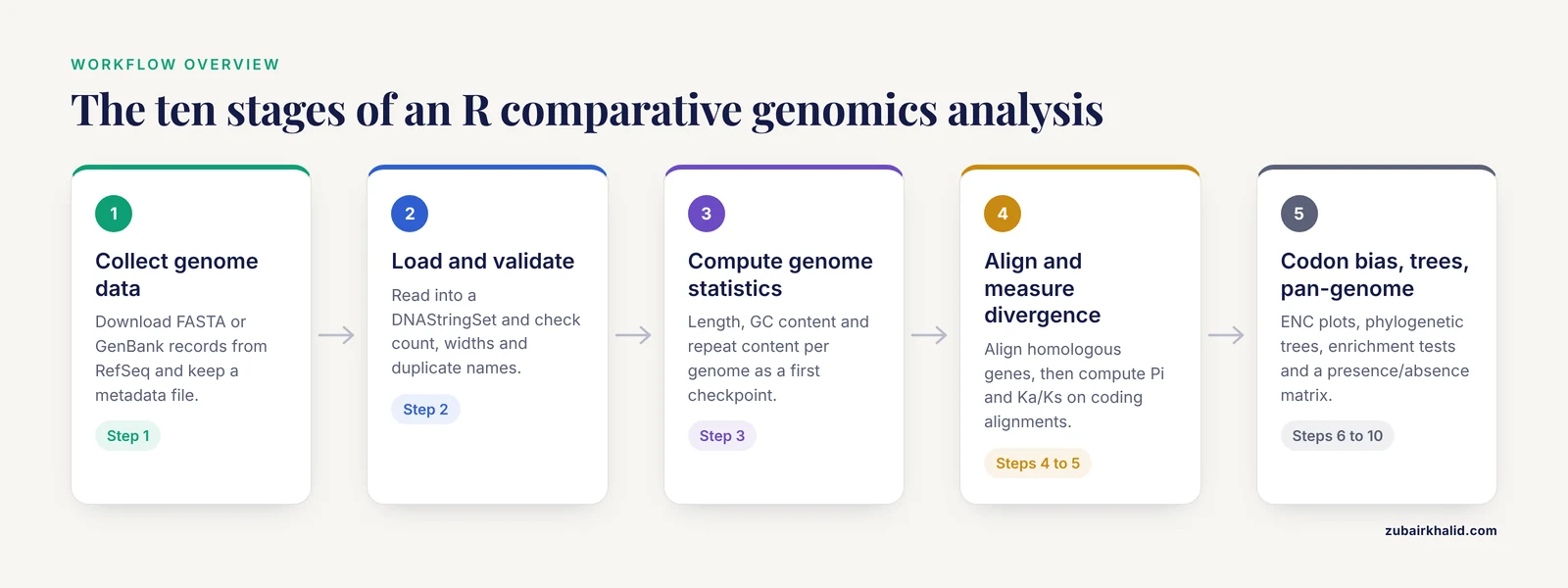
A comparative genomics analysis workflow in R has roughly ten stages, and you can run all of them from a single script or notebook:
- Collect genome sequences and annotation files in standard formats.
- Load sequences into R and validate them.
- Compute per-genome statistics such as length, GC content, and repeat content.
- Align homologous sequences across genomes.
- Quantify divergence with pairwise identity, nucleotide diversity, and Ka/Ks ratios.
- Analyze codon usage bias.
- Visualize gene order, synteny, and genome structure.
- Build phylogenetic trees from the distance or alignment data.
- Test functional enrichment for genes with unusual patterns.
- Assemble pan-genome or gene-family comparisons across many genomes.
Recent published comparative genomics studies map cleanly onto this structure. A study of the chloroplast genome of Rosa platyacantha reported genome length (157,133 bp), gene count (132), GC content (37.21%), repeat content (51 simple sequence repeats), codon usage bias, and nucleotide diversity hotspots across species comparisons [2]. A bacterial study of Rahnella sp. PAMC25617 combined genome-based phylogeny, average nucleotide identity, digital DNA-DNA hybridization, and pan-genomic analysis across 121 genomes to place an isolate in its evolutionary context [3]. Both papers follow the same underlying logic this workflow implements, one at the organellar scale and one at the bacterial whole-genome scale.
Choosing the Right Scale of Comparison
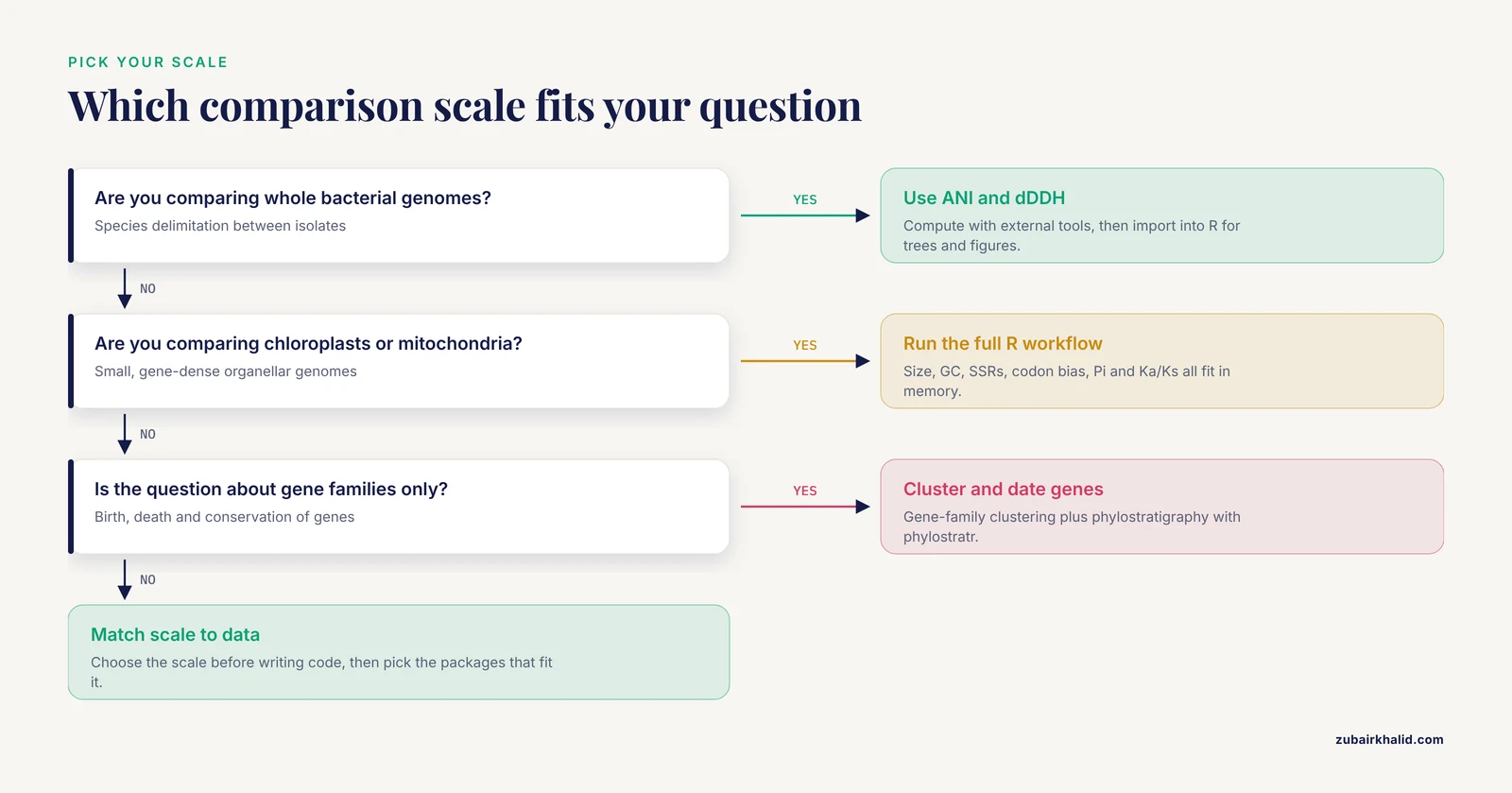
Comparative genomics is an umbrella term. Match the scale of your question to the scale of your data before writing any code.
Whole bacterial genomes. The standard comparison metrics are average nucleotide identity (ANI), the mean sequence identity shared between two genomes across their orthologous regions, and digital DNA-DNA hybridization (dDDH), an in silico estimate of genome-wide hybridization similarity. These metrics are used to decide whether isolates belong to the same species or represent distinct lineages, which is exactly how the Rahnella study used them [3]. ANI is usually computed with dedicated tools outside R, then imported into R for visualization and tree building.
Organellar genomes (chloroplasts, mitochondria). Chloroplast and mitochondrial genomes are small, gene-dense, and rich in structural features. Typical analyses cover genome size and gene content, repeat and simple sequence repeat (SSR) discovery, codon usage bias, RNA editing site prediction, nucleotide diversity (Pi) across regions, and Ka/Ks selection tests. The Rosa platyacantha study identified adaptive hotspots such as ycf3-trnS-GCU with a Pi value of 0.29005, along with trnC-GCA, trnT-UGU, and trnV-UAC, and found higher Pi in non-coding regions and in the large and small single-copy regions [2].
Gene families and protein sets. When the question concerns the birth, death, and conservation of genes rather than whole genomes, gene-family clustering and phylostratigraphy take over. Phylostratigraphic analysis assigns each protein an evolutionary origin based on the oldest lineage where a homolog appears, and the phylostratr R package exists precisely for this purpose [4].
The steps in this guide cover all three scales, with organellar genomes as the worked example because they fit comfortably in a laptop's memory.
Installing R, Bioconductor, and the Analysis Packages
Bioconductor is the main repository for genomics-specific R packages. Install it first, then install the packages this workflow uses:
install.packages("BiocManager")
BiocManager::install(c(
  "Biostrings",        # sequence containers and I/O
  "DECIPHER",          # sequence alignment and database tools
  "msa",               # interface to ClustalW, MUSCLE, ClustalOmega
  "coRdon",            # codon usage analysis
  "rtracklayer",       # GFF3 and BED annotation import
  "GenomicFeatures",   # transcript and gene coordinate objects
  "VariantAnnotation", # VCF parsing for SNP-level comparisons
  "ggtree"             # phylogenetic tree visualization
))

install.packages(c(
  "ape",       # phylogenetics and distance calculations
  "pegas",     # nucleotide diversity and population statistics
  "phangorn",  # phylogenetic model testing
  "seqinr",    # additional sequence utilities
  "gggenes",   # gene arrow visualization
  "micropan",  # pan-genome utilities
  "clusterProfiler", # functional enrichment
  "ggplot2"
))
If a package fails to install, check that your R version matches the current Bioconductor release. A common message looks like Bioconductor version 3.19 cannot be used with R 4.3. The fix is to update R itself, then rerun BiocManager::install(). This version coupling is deliberate. It is one of the mechanisms through which Bioconductor enforces reproducibility across the ecosystem [1].
Step 1: Collect Genome Data in Standard Formats
Before any R code runs, your inputs must be in a format R can read. The comparative genomics analysis workflow in R format question comes up constantly, so here is the mapping between file formats and the R functions that read them.
| Format | What it contains | R reader | Notes |
|---|---|---|---|
| FASTA (.fa, .fna) | Raw nucleotide or protein sequences | Biostrings::readDNAStringSet() or readAAStringSet() | The minimum input for alignment and statistics |
| GenBank (.gb, .gbk) | Sequence plus gene annotations | rtracklayer::import(format = "genbank") | Convenient when annotations matter |
| GFF3 (.gff, .gff3) | Gene, exon, and CDS coordinates | rtracklayer::import() | Pairs with a separate FASTA |
| VCF (.vcf, .vcf.gz) | Variant calls across samples | VariantAnnotation::readVcf() | Needed for SNP-level or LD comparisons |
| PLINK / HapMap | Genotype matrices | LDblockR reads these directly | Used in population-genomic comparisons |
| Newick (.nwk) | Tree topology | ape::read.tree() | Input or output for phylogenetic steps |
One lesson from recent tool development is that format heterogeneity is a real cost. The LDblockR toolkit was built specifically because common analysis programs require format conversion between VCF, HapMap, and PLINK files, so it unifies those inputs plus numeric 0/1/2 genotype matrices under one R-native object model [5]. When you design your own workflow, normalize to as few formats as possible at the start rather than converting repeatedly between steps.
Download genomes from NCBI's RefSeq or GenBank databases. For a chloroplast comparison, for example, you would download the complete chloroplast FASTA records for each species in your ingroup plus an outgroup. Name your files systematically, one FASTA per genome, and keep a spreadsheet or tab-delimited metadata file mapping file names to species, accession numbers, and source publications.
Step 2: Load Genomes and Check the Data
The workhorse container in Bioconductor is the DNAStringSet. Load your genomes and inspect them immediately:
library(Biostrings)

genomes <- readDNAStringSet("chloroplast_genomes.fasta")
genomes
Expected output for five chloroplast genomes:
DNAStringSet object of length 5:
    width seq                                          names
[6] 157133 ATGG...TTA                                   Rosa_platyacantha
[2] 155644 ATGG...TTA                                   Rosa_rugosa
[5] 156987 ATGG...TTA                                   Rosa_chinensis
[7] 155301 ATGG...TTA                                   Prunus_persica
[8] 155517 ATGG...TTA                                   Fragaria_vesca
Three checks matter here. First, the number of sequences should match the number of genomes you expected. Second, the widths should be plausible for your organism group. Chloroplast genomes cluster near 150,000 bp in most flowering plants, so a value of 40,000 bp signals a fragment or a mislabeled record. Third, scan names for duplicates or pathological characters. dist.dna() and several tree functions fail with a cryptic error when sequence names contain duplicates, so make them unique before proceeding:
names(genomes) <- make.unique(names(genomes))A frequent early failure is a path problem. The exact message Error in readDNAStringSet("chloroplast_genomes.fasta") : file does not exist means R's working directory does not contain the file. Run getwd() to see where R is looking and setwd() or a project-based workflow to fix it.
Step 3: Compute Basic Genome Statistics
Per-genome statistics anchor every later comparison and provide your first quality checkpoint.
gc_content <- function(x) {
  letterFrequency(x, "GC", as.prob = TRUE) * 100
}

stats <- data.frame(
  genome = names(genomes),
  length_bp = width(genomes),
  gc_percent = round(gc_content(genomes), 2)
)
stats
Example output on the toy dataset:
             genome length_bp gc_percent
1 Rosa_platyacantha    157133      37.21
2      Rosa_rugosa    155644      37.34
3   Rosa_chinensis    156987      37.28
4   Prunus_persica    155301      37.02
5  Fragaria_vesca    155517      36.98
This is where published values help you sanity-check your own. The R. platyacantha chloroplast genome is 157,133 bp with 37.21% GC content [2], and a bacterial Rahnella draft genome is 5.33 Mb with 52% GC [3]. If your computed values land far from published figures for the same species, suspect a truncation, contamination, or an assembly error before trusting anything downstream.
For repeat content, which matters greatly in plant mitogenomes, Biostrings::oligonucleotideFrequency() gives k-mer composition, and dedicated repeat finders handle SSR discovery. The relevance is easy to see from the literature. In one Brassicaceae mitogenome, transposable element sequence accounted for 21.83 kb (7.48% of the genome) and other repetitive DNA accounted for 44.03 kb (15.09%), and a regression across 32 mitogenomes showed a strong positive association between mitogenome size and transposable element content [6]. If you skip repeat characterization, you may misattribute genome size differences to gene content.
Step 4: Align Homologous Sequences
Comparative statistics require homologous positions, which means multiple sequence alignment. Two well-supported R routes exist.
Route A, DECIPHER, which is pure R and scales well:
library(DECIPHER)

rbcl <- readDNAStringSet("rbcl_genes.fasta")   # one homologous gene per genome
aligned <- AlignSeqs(rbcl)
aligned
Route B, the msa package, which wraps the classic aligners:
library(msa)

aln <- msa(rbcl, method = "Muscle")
aln
Expected output from msa:
MuscleMultipleAlignment with 5 rows and 1428 columns, 12 columns removed
aln-free
Details on row names and alignment are available as attributes
For protein-coding sequences, extract the coding regions first and confirm that each sequence length is an exact multiple of three before aligning codon-aware. The msa package also converts to the DNAbin format that the ape package expects:
library(ape)
aln_dnabin <- as.DNAbin(aligned)
A common error at this stage is Error in msa(...) : sequences must not contain gap characters. Remove pre-existing gaps or re-download clean sequences. Another frequent one, particularly with long organellar genomes, is memory exhaustion during full-genome alignment. Whole chloroplast or mitochondrial genomes often contain large rearrangements, so aligning whole genomes naively produces a poor result. The standard practice is to align shared genes individually, or to use a synteny-aware tool such as MUMmer or progressiveMauve outside R and import the resulting alignments.
Step 5: Measure Divergence Between Genomes
This is the analytical core. Three statistics cover most needs, and they answer different questions.
| Statistic | Question it answers | R function | Input |
|---|---|---|---|
| Pairwise identity | How similar are two aligned sequences? | seqinr or manual tabulation from alignment | Aligned sequences |
| Nucleotide diversity (Pi) | How variable is a region across taxa? | pegas::nucleotide.diversity() | Aligned DNAbin |
| Ka/Ks | Is a coding gene under purifying or diversifying selection? | ape::kaks() | Aligned CDS |
| ENC | How strong is codon usage bias? | coRdon::enc() | CDS sequences |
| ANI | Do two bacterial genomes belong to the same species? | External tools, imported into R | Whole genomes |
Nucleotide diversity. Pi is the average number of nucleotide differences per site between two sequences in a sample. Sliding-window Pi across an alignment localizes variable regions, which is how the Rosa study identified its adaptive hotspots such as ycf3-trnS-GCU with Pi = 0.29005 and found that non-coding regions carried higher diversity than coding regions [2].
library(pegas)

pi_total <- nucleotide.diversity(aln_dnabin)
pi_total
Expected output:
[6] 0.01845623To localize variation, compute Pi in windows using ape::NUV() or a manual split of the alignment into fixed-width bins, then plot Pi against position with ggplot2. Windows spanning intergenic spacers and tRNA-flanking regions deserve individual attention, since that is where hotspot loci tend to appear in plant organellar comparisons [2].
Ka/Ks. The Ka/Ks ratio compares the rate of nonsynonymous substitution per nonsynonymous site (Ka) to the rate of synonymous substitution per synonymous site (Ks). A ratio near zero indicates strong purifying selection, a ratio near one indicates neutral evolution, and a ratio above one suggests positive selection. One plant mitochondrial study found an elevated Ka/Ks ratio in the matR gene, flagging lineage-specific evolutionary dynamics for further site-model testing [7].
library(ape)

cds_aln <- read.dna("atpb_cds_alignment.fa", format = "fasta")
kk <- kaks(cds_aln)
kk$ka.ks      # pairwise Ka/Ks matrix
Expected output, as a lower-triangle matrix:
         seq1    seq2    seq3
seq1       NA      NA      NA
seq2  0.04812      NA      NA
seq3  0.05347 0.03199      NA
Two errors occur constantly here. The message Error in kaks(...) : sequences of different lengths means the CDS alignment was not codon-aware, so gaps inserted between codons corrupted the frame. Realign the coding sequences with a codon-aware method or trim the alignment to a multiple of three. A second issue is a warning about ambiguity codes or undefined Ks when two sequences are nearly identical, because Ks approaches zero and the ratio becomes unstable. Report those pairs with the component Ka and Ks values instead of the ratio alone.
Step 6: Analyze Codon Usage Bias
Codon usage bias measures the non-random use of synonymous codons, and it is a standard comparative genomics output. The effective number of codons (ENC) is the most common summary statistic, with values running from 20, meaning extreme bias toward one codon per amino acid, to 61, meaning no bias.
The coRdon package runs the full analysis on a set of coding sequences:
library(coRdon)

cds_set <- readDNAStringSet("cds_all_genomes.fasta")
cu <- codonUsage(cds_set)
enc_values <- enc(cu)
summary(enc_values)
Expected output:
   Min. 1st Qu.  Median    Mean 3rd Qu.    Max.
  29.10   32.85   34.40   34.62   36.10   45.20
Interpretation follows the literature closely. The R. platyacantha chloroplast study found a marked preference for synonymous codons ending in adenine or uracil (A/U) [2]. In a moss mitochondrial and chloroplast comparison, both organellar genomes showed the highest GC content at the first codon position, mitochondrial genes showed greater variation in ENC than chloroplast genes, and most genes clustered near the expected ENC curve, which is the standard test for whether mutational bias or selection drives the pattern [8]. A simple ENC-plot, ENC on the y axis against GC3 (GC content at third codon positions) on the x axis, tells you which side of that question your genes fall on. Genes below the expected ENC curve have codon bias beyond what GC3 alone explains.
Step 7: Visualize Genome Structure and Synteny
Synteny means conserved gene order across genomes. Plant organellar genomes rearrange frequently, so structural comparison carries real information. A Rhododendron mitochondrial study found its genome organized as two subgenomic linear molecules of 633,105 bp and 25,056 bp, detected six homologous segments representing 0.91% of the genome as evidence of interorganellar gene transfer, and used synteny analysis to confirm a close relationship with its congener while revealing structural divergence [7].
The gggenes package draws gene arrows in R, which is the cleanest way to render organelle gene maps:
library(gggenes)
library(ggplot2)

genes_df <- read.delim("gene_coordinates.tsv")   # genome, gene, start, end, strand
ggplot(genes_df, aes(xmin = start, xmax = end,
                     y = genome, fill = gene_class,
                     forward = strand == "+")) +
  geom_gene_arrow() +
  facet_wrap(~ genome, scales = "free_x", ncol = 1) +
  theme_genes()
For rearrangement detection and whole-genome synteny blocks, tools such as MUMmer and MCScanX remain the standard, and R's role is to parse their output and produce publication figures. This division of labor is normal. A workflow review notes that scripting languages like R are sufficient for small-scale, single-analyst pipelines, while large-scale comparisons benefit from combining R with external engines and formal workflow systems [9].
Step 8: Build Phylogenetic Trees From Your Comparisons
Phylogenetic trees summarize your comparative results into an explicit hypothesis of relationships. The ape package covers the standard route from alignment to tree:
library(ape)

dist_mat <- dist.dna(aln_dnabin, model = "TN93", pairwise.deletion = TRUE)
tree <- nj(dist_mat)

# Bootstrap support for internal branches
boot <- boot.phylo(tree, aln_dnabin,
                   function(x) nj(dist.dna(x, model = "TN93")),
                   B = 100, trees = TRUE)
tree$node.label <- as.character(round(boot$boot / 100, 2))
plot(tree, show.node.label = TRUE)
The TN93 model (Tamura-Nei 93) is a sensible default for organellar DNA because it allows different transition rates and unequal base frequencies. If dist.dna() returns Error : sequences of different lengths, your alignment collapsed to different widths per sequence, usually because of pairwise.deletion interacting with ragged gaps. Remove problematic columns globally or realign.
For bacteria, build the tree from imported ANI values instead. The Rahnella study placed its isolate using genome-based phylogeny together with ANI and dDDH, demonstrating that the isolate formed a distinct genomic lineage within its genus [3]. The R side of that analysis is simple:
ani <- read.delim("fastani_results.tsv")   # genome1, genome2, ani
ani_wide <- reshape(ani, idvar = "genome1", timevar = "genome2",
                    direction = "wide")
# Convert ANI to a distance and cluster
d <- as.dist(1 - as.matrix(ani_wide[, -1]) / 100)
ani_tree <- nj(d)
plot(ani_tree)
For publication figures, ggtree renders trees with annotations:
library(ggtree)
ggtree(tree) %<+% metadata_df + geom_tiplab() +
  geom_nodelab(aes(label = label), hjust = -0.05, size = 3)
Step 9: Annotate Function and Test Enrichment
When your comparison flags a set of genes, for example genes with elevated Ka/Ks or genes unique to one lineage, functional enrichment analysis places them in biological context. The clusterProfiler package is the standard R tool for over-representation analysis (ORA) and gene set enrichment analysis (GSEA), with bar plots, dot plots, and enrichment maps among its visual outputs [10].
library(clusterProfiler)

ego <- enrichGO(gene          = flagged_gene_ids,
                OrgDb         = org.At.tair.db,   # example: Arabidopsis
                keyType       = "TAIR",
                ont           = "BP",
                pAdjustMethod = "BH")
dotplot(ego, showCategory = 15)
The BH method refers to Benjamini-Hochberg correction, which controls the false discovery rate across the thousands of simultaneous term tests. A recent protocol extends this step with term-similarity networks exported to Cytoscape, including pie-chart networks that quantify pathway coverage and networks that carry expression directionality for each gene set [10]. That visualization layer matters when you have hundreds of enriched terms, which is common in genome-wide comparisons.
For a bacterial analysis, the same logic applies with COG or KEGG categories rather than Gene Ontology, and pan-genome studies routinely report the functional classification of accessory genes found in only a subset of genomes.
Step 10: Pan-Genome and Gene Family Comparison
A pan-genome is the union of all gene families found across a set of genomes. The core genome contains families present in every genome, the shell contains families present in some, and the cloud contains rare families. The Rahnella study framed its comparative analysis this way, comparing stress-response gene profiling across 121 genomes to separate conserved systems from lineage-specific ones [3].
The central data object is a presence/absence matrix, which you can build and explore in base R once gene families have been clustered with a tool such as MMseqs2 or OrthoFinder:
families <- read.delim("gene_clusters.tsv")   # columns: cluster, genome, gene

panmat <- table(families$cluster, families$genome) > 0
storage.mode(panmat) <- "numeric"

core_size   <- sum(rowSums(panmat) == ncol(panmat))
unique_to_i <- sum(rowSums(panmat) == 1)      # cloud-gene candidates
core_size
unique_to_i

library(pheatmap)
pheatmap(panmat, cluster_rows = TRUE, cluster_cols = TRUE,
         color = c("grey90", "steelblue"))
Expected console output on an illustrative five-genome dataset:
[6] 312
[6] 87
The heat map reveals lineage-specific blocks of accessory genes, and the micropan package fits accumulation curves that estimate how the pan-genome grows as genomes are added. On the gene-family evolution side, phylostratigraphy assigns each gene an age class based on its oldest detectable homolog. The MaizeGDB Phylostrata Tool applied this across 26 maize inbreds and found that more conserved proteins tend to be longer and more highly expressed, an example of how gene-age analysis connects comparative genomics to expression and function [4]. The phylostratr R package provides the underlying machinery for other species [4].
Turning the Script Into a Reusable Comparative Genomics Template
A one-off script is fine for exploration. A reusable comparative genomics analysis workflow in R template needs three additions, and current practice in workflow engineering is clear about why. Scripting languages and notebooks are sufficient for small, single-user pipelines, but shareable and maintainable pipelines require explicit structure, environment pinning, and modular stages [9].
- Pin your environment. Use
renv::init()andrenv::snapshot()so every collaborator installs the exact package versions you used. Bioconductor's strict R-to-Bioconductor version coupling helps here rather than hurts [1]. - Wrap each step as a target. The
targetspackage turns your numbered steps into a dependency graph so that changing one input reruns only the affected steps. This mirrors the modularity that formal workflow systems provide at larger scales [9]. - Document parameters in one configuration file. Keep window sizes, model choices, and file paths in a single YAML or CSV file that the script reads, so the template generalizes to the next dataset without code edits.
One caution about automating template generation. The mergen package uses large language models to generate and execute R analysis code from natural language prompts, with error feedback loops, and its evaluation found that LLMs handle some genomic analysis tasks well while other tasks require expert review of the generated code [11]. Treat any auto-generated analysis code the same way you treat your own drafts, as something to verify against known controls.
Common Mistakes and Limitations
Aligning whole genomes naively. Organellar and bacterial genomes with rearrangements produce meaningless alignments when processed as single sequences. Align shared genes separately or use a synteny-aware external aligner before importing into R.
Confusing paralogy with orthology. Gene families with recent duplications give inflated identity values if you align paralogs as if they were orthologs. Verify reciprocal best hits or use a proper ortholog inference tool before computing Ka/Ks.
Interpreting Ka/Ks from short or nearly identical sequences. When Ks approaches zero, the ratio explodes or becomes undefined. Report component rates for such pairs, and remember that a single elevated ratio, as in the matR case, is a signal for further site-model testing rather than a conclusion [7].
Using one normalization everywhere. Different downstream analyses call for different normalized representations of the same data. The microeco protocol for omics analysis explicitly selects different normalizations for different analysis stages based on best analytical practice [12], and the same principle applies to comparative genomics summaries.
Skipping the sanity checkpoints. Published GC contents, genome sizes, and gene counts for well-studied species exist precisely so you can validate your pipeline. The values reported in recent comparative studies, such as 37.21% GC for a rose chloroplast genome [2] or 45.3% GC for a Brassicaceae mitogenome [6], make excellent control targets.
Forgetting that R is not always the right engine. Whole-genome ANI computation, repeat discovery at scale, and pan-gene clustering typically run faster in dedicated command-line tools. R excels at statistics, integration, and visualization, and a clinical genomics review frames this correctly, noting R and Bioconductor's strengths in tool breadth and interoperability while acknowledging that heavyweight computation often lives elsewhere [1].
Assuming a workflow is reproducible because it runs. Reproducibility requires pinned versions, recorded parameters, and preserved inputs. Formal workflow systems were developed because ad hoc scripts fail this test at scale [9], and the same standards apply at laboratory scale.
Individual results from any comparative analysis depend on your specific species set, assembly quality, and annotation source, so treat published numbers as reference points rather than expectations your own data must match.
Frequently Asked Questions
Do I need command-line tools outside R for comparative genomics?
For small organellar genomes, no, R alone covers the full workflow. For whole bacterial genomes, you will typically compute ANI and cluster gene families with external tools such as FastANI and OrthoFinder, then import their results into R for statistics and visualization.
Which R packages handle FASTA and GenBank files?
Biostrings reads FASTA with readDNAStringSet() and readAAStringSet(), and rtracklayer imports GenBank and GFF3 annotation with import(). Together they cover nearly every format you will encounter in comparative genomics.
What is the difference between ANI and a phylogenetic tree?
ANI is a pairwise similarity percentage between two genomes, used mainly for species delimitation. A phylogenetic tree is a branching hypothesis of relationships across all taxa at once. Most analyses use both, because ANI quantifies closeness while the tree shows structure.
How many genomes do I need for a comparative analysis?
Two genomes support only pairwise comparisons. Pi, codon usage trends, and pan-genome curves become meaningful with roughly five or more genomes, and published pan-genomic studies often work with dozens to more than a hundred genomes.
Can R run pan-genome analysis for bacterial genomes?
Yes. The micropan package fits pan-genome accumulation curves, and the presence/absence matrix at the heart of pan-genomics is a simple table that base R computes and pheatmap visualizes. Gene-family clustering itself is faster in dedicated tools.
Why do my Ka/Ks values come out negative or undefined?
Ks near zero makes the ratio unstable, and unaligned codon frames corrupt the site counts. Check that the coding alignment length is a multiple of three, remove sequences with many ambiguity codes, and report Ka and Ks separately for very close pairs.
How do I make the workflow reproducible?
Pin package versions with renv, encode each step as a targets target, and keep all parameters in one configuration file. Formal workflow research identifies environment pinning and modularity as the requirements that plain scripts usually miss.
Is R fast enough for whole-genome comparisons?
R handles chloroplast and mitochondrial genomes and gene-level comparisons comfortably. Genome-scale alignment and ANI computation belong in compiled external tools, with R handling the statistical analysis and figures on the imported results.
Sources
- Using R and Bioconductor in Clinical Genomics and Transcriptomics.
- Characteristics, comparative genomics, and phylogenetic analysis of the chloroplast genome of Rosaplatyacantha.
- Comparative genomic analysis of Rahnella sp. PAMC25617 isolated from cryoconite reveals a glutathione-dependent formaldehyde detoxification pathway.
- MaizeGDB Phylostrata Tool: exploring evolutionary origins of maize proteins.
- LDblockR: a cross-platform R toolkit for multi-format linkage disequilibrium analysis and integrated regional genomics visualization.
- Mitochondrial Genome of the Korean Endemic Arabis takesimana (Brassicaceae): Addition to the Genomic Resources and Evolutionary Insights.
- Characterization of the complete mitochondrial genome of Rhododendron simsii var. putuoense and its comparative evolutionary analysis.
- Mitochondrial Genome Characteristics of Rhodobryum laxelimbatum and Comparative Analysis of RNA Editing and Codon Usage Bias With the Chloroplast Genome.
- Developing and reusing bioinformatics data analysis pipelines using scientific workflow systems.
- Enhancing Interpretation of Functional Enrichment Analysis Results with Advanced Network Visualizations.
- Leveraging large language models for data analysis automation.
- A workflow for statistical analysis and visualization of microbiome omics data using the R microeco package.