How to Visualize Copy Number Variations (CNVs) in R
By Dr. Zubair Khalid, DVM, MS, PhD ·

By the end of this guide you will build four kinds of CNV plot in R from a single segmentation table: a genome-wide copy number profile, a per-chromosome plot with genes labeled, a multi-sample heatmap that clusters samples by copy number pattern, and an interactive Shiny browser. Every example is self-contained and runs on a laptop with R 4.2 or newer, so you can reproduce each figure before your own data arrives.
You need two things on hand. The first is R with the packages listed below. The second is a segmentation table with chromosome, start, end, and a copy number or log2 value from any caller or pipeline. If you have no data yet, the worked example includes a small synthetic profile that stands in for one.
Copy number variation (CNV) is a gain or a loss of a stretch of DNA relative to a reference genome. A tumor with three copies of a region that is normally present in two copies carries a single-copy gain, and a region present in one copy carries a heterozygous loss. R for bioinformatics handles this problem well because the ggplot2 grammar and the tidyverse produce the layered look a CNV profile needs, a combination used across published genomics analyses [1], while Bioconductor supplies genomics-aware packages and data structures. The plotting step matters because callers emit long candidate lists that need visual triage before anyone acts on them, a reality that pushed clinical genomics groups to build dedicated review interfaces [2].
What a CNV Plot Actually Shows
Most sequencing-based CNV callers follow one logic. They cut the genome into fixed windows called bins, count read depth (the number of sequencing reads overlapping each bin), compare it to an expected value from a reference, and take the log2 of that ratio. A log2 ratio of 0 means neutral, positive means gain, and negative means loss. A segmentation algorithm then merges neighboring bins that share a consistent level into segments, each with one start, one end, and one copy number estimate. Older technologies such as fluorescence in situ hybridization and array comparative genomic hybridization resolved these events more coarsely, which is one reason read-depth methods built on next-generation sequencing displaced them [3].
That two-level structure defines what a CNV plot can show. Bin-level points expose noise, waves, and variance. Segment lines expose the calls. The workflow below draws both, and the quality control section explains why the overlay is the single most useful diagnostic you can produce.
Methods differ under the hood. A benchmark comparison of six callers, CNV-seq, FREEC, readDepth, CNVnator, SegSeq, and event-wise testing, evaluated sensitivity and specificity with ROC curves (sensitivity plotted against specificity across thresholds), breakpoint and copy number accuracy with box plots, and consistency between methods with Venn diagrams and F-scores (the harmonic mean of precision and recall) [3]. The practical lesson for plotting is that two callers can disagree about the same region, so a good figure makes confidence visible instead of hiding it.
Low-pass whole genome sequencing (LP-WGS), which sequences at low coverage specifically to infer copy number, is now a common source of such data, and end-to-end pipelines wrap quality control, CNV calling, CNV plots, and segmentation files with statistics into a single command [4]. If your data comes from such a pipeline, its segmentation file is exactly the input the code below expects.
Setting Up Your R Environment
Install CRAN packages with install.packages(). Bioconductor, the open-source project that hosts most of R's genomics infrastructure, distributes its packages through BiocManager.
install.packages(c("ggplot2", "dplyr", "tidyr", "readr", "tibble",
                   "ggrepel", "shiny"))

if (!requireNamespace("BiocManager", quietly = TRUE)) {
  install.packages("BiocManager")
}
BiocManager::install(c("GenomicRanges", "maftools", "circlize", "ComplexHeatmap"))
If you call library(ComplexHeatmap) before installing it, R answers "there is no package called 'ComplexHeatmap'". Running install.packages("ComplexHeatmap") instead of BiocManager::install() typically answers that the package "is not available", because Bioconductor-only packages are not on CRAN.
| Package | Source | Role in a CNV plot |
|---|---|---|
| , - | , - | , - |
| ggplot2 | CRAN | plotting grammar for profiles and per-chromosome figures |
| dplyr, tidyr, readr, tibble | CRAN | importing and reshaping segmentation tables |
| ggrepel | CRAN | gene labels that do not collide |
| GenomicRanges | Bioconductor | overlaps between segments and genes |
| maftools | Bioconductor | GISTIC-style copy number summaries [5] |
| circlize | Bioconductor | circos plots and color ramps |
| ComplexHeatmap | Bioconductor | multi-sample heatmaps |
| shiny | CRAN | interactive browsers [6] |
If you work from VCF files (the standard text format for variant calls), vcfR reads them into R and pairs naturally with maftools for visualization, a combination that existing Shiny-based viewers build on [5].
Understanding the Input: Segmentation Files and Bin Ratios
A segmentation file is a table with at least four columns: chromosome, start, end, and a copy number estimate or log2 value. Pipelines add per-segment statistics and per-sample summaries [4]. Bin-level files have the same shape at finer resolution. Coordinates refer to a genome build, the reference coordinate system such as GRCh37 (hg19) or GRCh38 (hg38), and every file in one analysis should use the same build. Read real files with readr and rename columns to a common set:
library(readr)

seg <- read_tsv("sample_A_segments.tsv") %>%
  rename(chromosome = chrom, start = start_pos,
         end = end_pos, cn = copy_number)
For this tutorial, an artificial profile keeps every number predictable. It encodes a single-copy gain on 1p, a loss of all of chr2, a high-level gain on most of chr7, and a heterozygous deletion on 17p. Chromosome lengths are approximate GRCh37 (hg19) values in bases.
library(tibble)

seg <- tribble(
  ~chromosome, ~start,     ~end,       ~cn,
  "chr1",      1,          65000000,   3,
  "chr1",      65000001,   249250621,  2,
  "chr2",      1,          243199373,  1,
  "chr3",      1,          198022430,  2,
  "chr7",      1,          25000000,   2,
  "chr7",      25000001,   159138663,  4,
  "chr17",     1,          7600000,    1,
  "chr17",     7600001,    81695210,   2
)
seg
Expected output:
# A tibble: 8 × 4
  chromosome      start        end    cn
  <chr>          <dbl>      <dbl> <dbl>
1 chr1               1   65000000     3
2 chr1        65000001  249250621     2
3 chr2               1  243199373     1
4 chr3               1  198022430     2
5 chr7               1   25000000     2
6 chr7        25000001  159138663     4
7 chr17              1    7600000     1
8 chr17       7600001   81695210     2
Segments tile each chromosome with no gaps, which is what most callers emit. A one-base gap will not break the plot, but unsorted or missing chromosomes will, as the mistakes section shows.
Building a CNV Plot in R, Step by Step
Step 1: Load the libraries
library(ggplot2)
library(dplyr)
Step 2: Order chromosomes and compute genome offsets
A genome-wide plot lays chromosomes end to end on one x axis. Each chromosome needs an offset equal to the combined length of every chromosome before it. Build the lookup table once and reuse it for every figure in a project.
chr_len <- c("chr1"  = 249250621,
             "chr2"  = 243199373,
             "chr3"  = 198022430,
             "chr7"  = 159138663,
             "chr17" =  81695210)

chr_tbl <- tibble(chromosome = factor(names(chr_len), levels = names(chr_len)),
                  chr_len    = as.numeric(chr_len)) %>%
  mutate(offset = lag(cumsum(chr_len), default = 0))

chr_tbl
Expected output:
# A tibble: 5 × 3
  chromosome    chr_len    offset
  <fct>          <dbl>     <dbl>
1 chr1       249250621         0
2 chr2       243199373 249250621
3 chr3       198022430 492449994
4 chr7       159138663 690472424
5 chr17       81695210 849611087
For a full karyotype view, list every chromosome from chr1 through chr22 plus X and Y in chr_len, and the axis will reserve ordered space for each. The factor() call is what blocks alphabetical sorting.
Step 3: Convert copy number to log2 and label states
plot_df <- seg %>%
  mutate(chromosome = factor(chromosome, levels = levels(chr_tbl$chromosome))) %>%
  left_join(chr_tbl, by = "chromosome") %>%
  mutate(
    log2         = log2(cn / 2),
    genome_start = start + offset,
    genome_end   = end + offset,
    genome_mid   = (genome_start + genome_end) / 2,
    state = case_when(
      cn == 0 ~ "homozygous deletion",
      cn == 1 ~ "heterozygous deletion",
      cn == 2 ~ "neutral",
      cn >= 3 ~ "amplification"
    )
  )

plot_df %>% select(chromosome, start, end, cn, log2, offset, state)
Expected output:
# A tibble: 8 × 7
  chromosome      start        end    cn   log2    offset state
  <fct>          <dbl>      <dbl> <dbl>  <dbl>     <dbl> <chr>
1 chr1               1   65000000     3  0.585         0 amplification
2 chr1        65000001  249250621     2  0             0 neutral
3 chr2               1  243199373     1 -1             0 heterozygous deletion
4 chr3               1  198022430     2  0             0 neutral
5 chr7               1   25000000     2  0             0 neutral
6 chr7        25000001  159138663     4  1             0 amplification
7 chr17              1    7600000     1 -1             0 heterozygous deletion
8 chr17       7600001   81695210     2  0             0 neutral
The conversion assumes a diploid reference, so copy number 3 maps to log2(3/2) = 0.58, copy number 1 maps to -1, and copy number 4 maps to 1. The state column exists to drive colors and nothing else.
Step 4: Draw the genome-wide profile
cn_cols <- c("homozygous deletion"   = "#67000d",
             "heterozygous deletion" = "#fb6a4a",
             "neutral"               = "grey65",
             "amplification"         = "#2171b5")

p <- ggplot(plot_df, aes(x = genome_mid, y = log2)) +
  geom_hline(yintercept = 0, color = "grey30", linetype = "dashed") +
  geom_hline(yintercept = c(log2(3/2), log2(1/2)),
             color = c("#2171b5", "#cb181d"), linetype = "dotted") +
  geom_segment(aes(x = genome_start, xend = genome_end,
                   y = log2, yend = log2, color = state),
               linewidth = 2.5) +
  scale_x_continuous(breaks = chr_tbl$offset + chr_tbl$chr_len / 2,
                     labels = as.character(chr_tbl$chromosome),
                     expand = c(0.01, 0)) +
  scale_y_continuous(name = "log2 copy ratio",
                     sec.axis = sec_axis(~ 2 * 2^.x,
                                         name = "copy number (ploidy 2)")) +
  scale_color_manual(values = cn_cols, name = NULL) +
  theme_minimal(base_size = 12) +
  theme(panel.grid.minor = element_blank())

p
What you should see: gray bars at 0 for the neutral regions, a blue bar at about 0.58 across the first 65 million bases of chr1, a salmon bar at -1 spanning all of chr2, a blue bar at 1.0 over most of chr7, and a dark red bar at -1 on the left arm of chr17. A dashed line marks 0 and dotted guides mark +0.58 and -1. The right axis converts log2 back to copy number, which reviewers tend to appreciate.
Three parameters carry the figure. linewidth sets bar thickness and replaced the old size argument in ggplot2 3.4.0. The sec_axis formula, ~ 2 * 2^.x, is the inverse of the log2 conversion and is correct only when the reference ploidy is 2, so change both together for a triploid baseline. The named values vector in scale_color_manual keeps every state the same color in every figure of a paper.
Step 5: Save the figure
ggsave("cnv_genome_wide.pdf", p, width = 10, height = 3.5)
ggsave("cnv_genome_wide.png", p, width = 10, height = 3.5, dpi = 300)
PDF keeps long thin segments crisp at any zoom. The 300 dpi PNG is for slides.
Per-Chromosome Plots with Gene Annotation
Genome-wide profiles answer "where". Per-chromosome plots answer "which gene". The 17p deletion in the example covers the TP53 locus, and a reviewer will want that labeled. ggrepel keeps labels from overlapping, and it belongs to the same tidyverse toolkit, alongside ggplot2, dplyr, and tidyr, that published genomics analyses routinely use for visualization [1].
library(ggrepel)

genes <- tribble(
  ~chromosome, ~start,  ~end,     ~gene,
  "chr17",     7512000, 7532000,  "TP53"    # approximate hg19 coordinates
)

chr17 <- filter(plot_df, chromosome == "chr17")

ggplot(chr17, aes(x = start, y = log2)) +
  geom_segment(aes(x = start, xend = end, y = log2, yend = log2, color = state),
               linewidth = 4) +
  geom_rect(data = genes,
            aes(xmin = start, xmax = end, ymin = -1.18, ymax = -0.82),
            fill = "black", alpha = 0.35, inherit.aes = FALSE) +
  geom_text_repel(data = genes,
                  aes(x = (start + end) / 2, y = -1, label = gene),
                  inherit.aes = FALSE, size = 4, direction = "x") +
  scale_color_manual(values = cn_cols, name = NULL) +
  labs(x = "Position on chr17 (bases)", y = "log2 copy ratio") +
  theme_minimal(base_size = 12)
The black rectangle marks the gene body inside the deletion, and geom_text_repel places the name without covering the bar. Pass a whole gene table rather than one row when dozens of genes need labels.
To assign genes to segments programmatically, use GenomicRanges instead of eyeballing coordinates.
library(GenomicRanges)

segs_gr <- GRanges(as.character(plot_df$chromosome),
                   IRanges(plot_df$start, plot_df$end),
                   cn = plot_df$cn)
genes_gr <- GRanges(genes$chromosome,
                    IRanges(genes$start, genes$end),
                    gene = genes$gene)

as.data.frame(findOverlaps(segs_gr, genes_gr))
Expected output:
  queryHits subjectHits
1         7           1
Query hit 7 is the seventh segment, the chr17 deletion, and it overlaps subject hit 1, TP53. That two-column table is the bridge between a CNV plot and a candidate gene list.
Multi-Sample Heatmaps of Copy Number
A single profile hides cohort structure. A heatmap with bins as rows and samples as columns shows which events are shared, and clustering the columns groups samples with matching aneuploidy, meaning gains or losses of whole chromosomes or chromosome arms, an approach that CNV pipelines build in as sample clustering by copy number pattern [4].
If your data is a long table with one row per sample per bin, reshape it to a matrix first.
library(tidyr)

cnv_mat <- bins_long %>%
  select(bin_id, sample, log2) %>%
  pivot_wider(names_from = sample, values_from = log2) %>%
  tibble::column_to_rownames("bin_id") %>%
  as.matrix()
For a self-contained demo, simulate twelve samples with two shared events.
library(circlize)
library(ComplexHeatmap)

set.seed(7)
bins    <- 400
samples <- sprintf("sample_%02d", 1:12)
cnv_mat <- matrix(rnorm(bins * length(samples), sd = 0.12),
                  nrow = bins, dimnames = list(NULL, samples))
cnv_mat[  80:120,  1:4]  <- cnv_mat[  80:120,  1:4]  + 0.7   # shared gain
cnv_mat[ 260:330,  9:12] <- cnv_mat[ 260:330,  9:12] - 1.0   # shared loss

col_fun <- colorRamp2(c(-1.5, 0, 1.5), c("#2166ac", "white", "#b2182b"))

Heatmap(cnv_mat,
        col            = col_fun,
        name           = "log2",
        cluster_rows   = FALSE,
        show_row_names = FALSE,
        row_title      = "Genomic bins (ordered by position)",
        column_title   = "Samples clustered by CNV pattern")
Expected result: the column dendrogram splits off samples 01 to 04, which share a blue block at bins 80 to 120, and samples 09 to 12, which share a red block at bins 260 to 330. The remaining four look flat and gray. The color function is anchored so that 0 is white, which keeps neutral regions visually quiet. With millions of bins, aggregate to segments first, or the heatmap takes minutes to render and loses its message.
Interactive CNV Plots with Shiny
Static figures answer the questions you anticipated. Interactive ones answer the questions reviewers ask instead. Shiny, R's framework for web apps, is the standard route and powers real genomics tools, from an educational yeast evolution browser organized around an interactive chromosome map, mutation-type graphs, and a gene viewer [6], to a VCF summarization app that wraps vcfR and maftools behind buttons and menus [5].
A minimal browser reuses plot_df and cn_cols from the steps above. Define both before shinyApp() runs, or the app opens with an "object 'plot_df' not found" error.
library(shiny)

ui <- fluidPage(
  titlePanel("CNV browser"),
  selectInput("chr", "Chromosome:",
              choices = c("All", levels(plot_df$chromosome))),
  plotOutput("profile", brush = "brush", height = "300px"),
  tableOutput("selected")
)

server <- function(input, output, session) {
  output$profile <- renderPlot({
    d <- if (input$chr == "All") plot_df else filter(plot_df, chromosome == input$chr)
    ggplot(d, aes(x = genome_start, y = log2)) +
      geom_segment(aes(x = genome_start, xend = genome_end,
                       y = log2, yend = log2, color = state),
                   linewidth = 2) +
      geom_hline(yintercept = 0, linetype = "dashed", color = "grey40") +
      scale_color_manual(values = cn_cols, name = NULL) +
      theme_minimal()
  })

  output$selected <- renderTable({
    brushedPoints(plot_df, input$brush,
                  xvar = "genome_start", yvar = "log2")
  })
}

shinyApp(ui, server)
Drag a box across any segment and the table below the plot lists its chromosome, coordinates, copy number, and log2 value. That brush-to-table pattern is the core of most CNV review apps, including purpose-built clinical environments that replace long call lists with visual summaries designed for at-a-glance relevance judgments [2].
Ready-Made Alternatives: maftools and circlize
Sometimes the plot already exists. If your CNV results come from GISTIC, a widely used tool for scoring recurrent copy number alterations across many samples, maftools reads the standard output files and draws chromosome-scale summaries in two lines [5].
library(maftools)

gistic <- readGistic(
  gisticAllLesionsFile = "all_lesions.conf_99.txt",
  gisticAmpGenesFile   = "amp_genes.conf_99.txt",
  gisticDelGenesFile   = "del_genes.conf_99.txt",
  isTCGA = FALSE
)

gisticChromPlot(gistic)
The three input files are the standard GISTIC outputs, and isTCGA = TRUE applies TCGA-style sample name cleanup when your data comes from that resource. maftools function names shift between versions, so open ?gisticChromPlot if a call fails.
For a circular genome view, circlize wraps copy number tracks around an ideogram, a schematic chromosome map with cytoband shading.
library(circlize)

bed <- as.data.frame(plot_df)[, c("chromosome", "start", "end", "log2")]

circos.initializeWithIdeogram(chromosomes = as.character(unique(bed$chromosome)))
circos.genomicTrack(bed, track.height = 0.12,
                    panel.fun = function(region, value) {
                      circos.genomicLines(region, value, type = "h",
                                          col = ifelse(value$log2 >= 0,
                                                       "#b2182b", "#2166ac"))
                    })
circos.clear()
Circos figures reward iteration, and every attempt should end with circos.clear(). Without it, the next plot stacks tracks on the old canvas and produces overlapping nonsense.
Key Formulas and Plot Options at a Glance
| Quantity or option | Formula or setting | Worked value |
|---|---|---|
| , - | , - | , - |
| log2 copy ratio | log2(sample CN / reference CN) | CN 3 in a diploid reference: log2(3/2) = 0.58 |
| Copy number from log2 | CN = ploidy × 2^log2 | log2 = 1 at ploidy 2 gives CN 4 |
| Heterozygous loss | log2(1/2) | -1.00 |
| Homozygous loss | log2(0/2) | -Inf, cap at -4 for display |
| Purity-adjusted expectation | log2((p × CN + (1 - p) × 2) / 2) | CN 4 at purity 0.6: log2(1.6) = 0.68 |
| Chromosome offset | sum of lengths of all earlier chromosomes | chr2 offset in hg19: 249,250,621 bases |
| Line thickness | linewidth (ggplot2 3.4.0 or newer) | linewidth = 2.5 |
| Diverging color midpoint | 0 on the log2 scale | colorRamp2(c(-1, 0, 1), c("blue", "white", "red")) |
| Publication export | ggsave(file, plot, width, height, dpi) | 10 by 3.5 inches, 300 dpi |
Tips for Checking That the Plot Tells the Truth
A CNV plot can be beautiful and wrong. Fold these checks into the routine.
- Overlay bins on segments. If you have a bin-level table with genome_start and log2, built with the same offsets, draw the points faintly and the segments on top.
ggplot(mapping = aes(x = genome_start, y = log2)) +
  geom_point(data = bins_df, alpha = 0.15, size = 0.3, color = "grey45") +
  geom_segment(data = plot_df,
               aes(x = genome_start, xend = genome_end, y = log2, yend = log2),
               color = "red", linewidth = 1)
If the red line does not track the center of the point cloud, the segmentation is off, or the bins carry a systematic bias such as a GC-content wave.
- Plot a control sample first. A matched normal or a known-diploid sample should be a flat gray band around 0. Waves in the control mean a library or GC problem that will contaminate every sample drawn after it.
- Cross-check important calls. The multi-caller benchmark discussed earlier measured real differences in sensitivity, specificity, breakpoint accuracy, and copy number accuracy across methods [3]. An event supported by two independent callers, or by an orthogonal assay, deserves a bolder box than an event supported by one.
- Respect resolution. Low-coverage sequencing detects large aneuploidies and supports genome-wide summaries such as the fraction of the genome that is non-euploid, but the same low coverage that makes it cheap limits how small an event it can resolve [4]. A few-kilobase deletion is invisible at 100-kilobase bins no matter how the plot is styled.
- Route borderline calls to visual review. In clinical genomics, automated CNV calls are treated as candidates, and human review separates relevant findings from the rest, which is why dedicated visual review environments were built for this task [2]. Annotate on the figure whatever a reviewer would otherwise ask about.
Common Mistakes and Limitations
- Alphabetical chromosome order. Symptom: the x axis reads chr1, chr10, chr11, chr2, chr20. Cause: chromosomes stored as character strings sort lexicographically. Fix: convert the column to a factor with karyotype-ordered levels before plotting, as Step 2 does. Every axis break inherits the fix.
- Infinite values from homozygous deletions. log2(0/2) is -Inf, and ggplot2 drops infinite values with a warning like "Removed 2 rows containing missing or infinite values (
geom_segment())." The deletion you care about most is the one that vanished. Fix: cap before plotting, for example mutate(log2 = ifelse(is.infinite(log2), -4, log2)), and state the floor in the caption as a display choice.
- Using size instead of linewidth. Since ggplot2 3.4.0, line thickness in geom_segment and geom_line is set by linewidth, and passing size triggers "Using the
sizeaesthetic with lines was deprecated in ggplot2 3.4.0. Please use thelinewidthaesthetic instead." The plot still renders today and breaks later when the compatibility shim disappears. Fix the argument name now.
- Mixing genome builds. A segmentation file in GRCh37 (hg19) coordinates plotted against gene models in GRCh38 (hg38) shifts segments by amounts that vary by chromosome, sometimes by tens of millions of bases, so genes appear to sit outside the events that contain them. Symptom: a deletion that clearly covers a gene in a genome browser misses it in your figure. Fix: lift over one side to match the other, or re-call everything in one build, and record the build in the caption.
- Ignoring purity and ploidy. In a sample that is 60 percent tumor cells, a true four-copy gain does not sit at log2(4/2) = 1. It sits at log2((0.6 × 4 + 0.4 × 2) / 2) = log2(1.6), about 0.68. Purity dilutes amplitude, and whole-genome doubling shifts the baseline, so a fixed vertical threshold misclassifies events. Fix: estimate purity and ploidy where possible, adjust the reference level, and annotate both on the figure.
- Overplotting bin-level data. Whole-genome bin files can hold millions of rows, and a PDF with that many points can reach hundreds of megabytes. Fix: draw segments as lines, downsample neutral bins, set alpha below 0.3, or rasterize points with the ggrastr package, and draw segments last so they sit on top.
- Treating caller output as settled truth. Caller performance varies, and low-coverage data resolves large events better than focal ones. Fix: report the caller, bin size, and genome build behind every figure, and validate events that matter with a second method.
Preparing Messy Real-World Caller Output for Plotting
The tutorial uses a hand-built tribble, which is honest about its own schema. Real files are not. Every major caller and pipeline emits segmentation output with different column names, different coordinate conventions, and different ways of representing missing values, and the plotting code in this guide assumes four tidy columns. The first practical step of any CNV figure is therefore a normalization script, not a ggplot call.
A typical raw file might arrive with columns like chr, start_hg19, end_hg19, copynumber, plus extra statistics you do not need for the plot. Normalize it once, at import, and every downstream figure inherits the fix:
library(readr)
library(dplyr)

raw <- read_csv("caller_output.csv",
                na = c("", "NA", "N/A", "n/a", "."))

seg_raw <- raw %>%
  transmute(
    chromosome = as.character(chr),
    start      = as.numeric(start_hg19),
    end        = as.numeric(end_hg19),
    cn         = as.numeric(copynumber)
  )
Three details in that block prevent the most common import failures. First, na = c("", "NA", "N/A", "n/a", ".") tells readr which strings mean missing; without it, a single n/a cell silently turns the whole cn column into text, and downstream arithmetic fails with a type error. Second, transmute() drops everything except the four plotting columns, so leftover statistics cannot collide with names you create later such as log2 or state. Third, everything is coerced explicitly with as.numeric(), which fails loudly during import rather than mysteriously during plotting.
Chromosome naming is its own trap. Some callers write 1, others chr1, and some write chr23 for the X chromosome. Pick one convention, ideally the chr-prefixed form that matches your annotation resources, and enforce it:
seg_raw <- seg_raw %>%
  mutate(chromosome = if_else(grepl("^chr", chromosome),
                              chromosome,
                              paste0("chr", chromosome)),
         chromosome = recode(chromosome,
                             "chr23" = "chrX",
                             "chr24" = "chrY",
                             "chrM"  = "chrMT"))
Then verify the result against the chromosome table you built for the plot. Any name in the data that the plot does not know is a defect worth catching before the figure:
setdiff(unique(seg_raw$chromosome), names(chr_len))If that returns "chr5" when your lookup only contains five chromosomes, either the lookup is incomplete or the caller emitted something unexpected, and both are better discovered now than as an empty facet later.
Decide explicitly what happens to the sex chromosomes and the mitochondrial chromosome. Read-depth CNV callers behave differently on chrX and chrY because of dosage compensation and male versus female reference baselines, and many pipelines exclude them or treat them as special cases [4]. For a first figure, filtering them out with filter(!chromosome %in% c("chrX", "chrY", "chrMT")) is defensible; for a figure that will be reviewed clinically, keeping them with an explicit note about how they were handled is better than silently dropping them. Either way, the decision belongs in a comment next to the filter, not in the head of whoever reads the figure six months later.
Validating Segmentation Tables Before You Plot
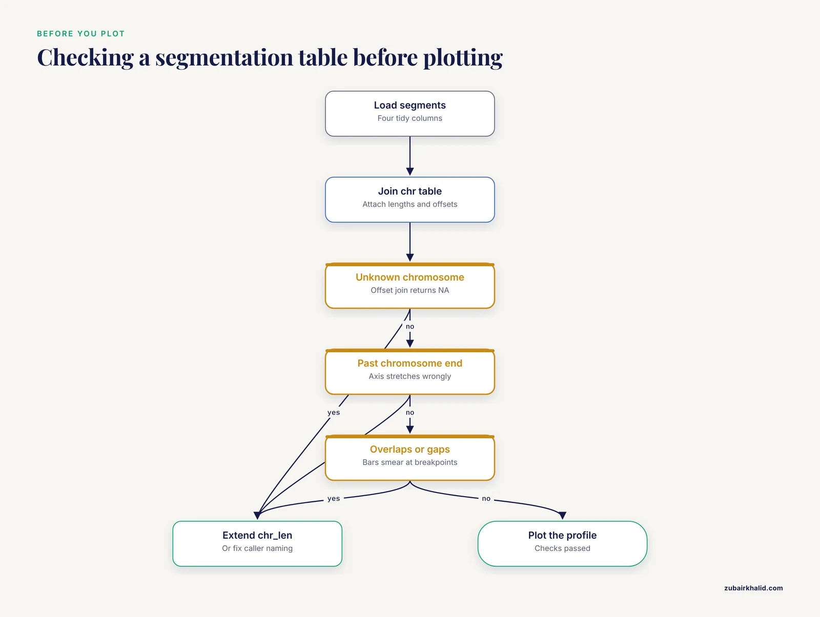
Most broken CNV figures are not ggplot problems. They are data problems that ggplot exposes in confusing ways. A five-line validation step converts vague plotting symptoms into concrete data complaints.
Segmentation tables can fail in four ways that matter for plotting: coordinates that run past the end of a chromosome, segments that overlap, unexplained gaps, and missing copy number values. The function below reports all of them in one pass:
check_segments <- function(seg, chr_tbl) {
  seg %>%
    mutate(chromosome = as.character(chromosome)) %>%
    left_join(chr_tbl, by = "chromosome") %>%
    group_by(chromosome) %>%
    arrange(start, .by_group = TRUE) %>%
    mutate(prev_end  = lag(end),
           gap_bases = start - prev_end - 1) %>%
    ungroup() %>%
    summarise(
      chromosomes_unknown   = sum(is.na(chr_len)),
      beyond_chromosome_end = sum(end > chr_len, na.rm = TRUE),
      reversed_segments     = sum(end < start, na.rm = TRUE),
      overlaps              = sum(gap_bases < -1, na.rm = TRUE),
      gaps                  = sum(gap_bases > 0, na.rm = TRUE),
      missing_cn            = sum(is.na(cn))
    )
}

check_segments(seg, chr_tbl)
Each summary column maps to a specific plotting symptom. chromosomes_unknown greater than zero predicts a factor level warning and an invisible chromosome on the x axis, because the offset join returns NA and ggplot drops those segments silently. beyond_chromosome_end stretches the axis past the last chromosome's label and makes chromosome 17, say, look wider than chromosome 1. overlaps makes segment bars stack into an unreadable dark smear at breakpoints. gaps is the least alarming: most callers emit contiguous tiles, but some leave one-base gaps between adjacent segments, and the tutorial's own profile tolerates them. The comparison uses -1 rather than 0 precisely so that touching segments are not flagged as overlaps.
Run this check on every sample before plotting, not only the first. Batch effects show up here: if sample 12 is the only one with gaps in its segmentation, the problem is in that sample's processing, and no amount of plot styling will hide it.
One more check costs almost nothing and prevents a classic silent failure. Confirm that every chromosome is present for every sample in a multi-sample analysis:
seg %>%
  count(chromosome, name = "n_segments") %>%
  anti_join(chr_tbl, by = "chromosome")
A chromosome that appears in nine samples and not the tenth usually means a failed call or an empty segmentation file for that sample, and the faceted plots in the next section will render it as a blank panel unless you catch it here.
Turning the Tutorial Code into a Reusable Plotting Function
The step-by-step profile in the main guide is written for one table. A real project plots dozens of samples, and copy-pasting the pipeline per sample guarantees that one sample's figure silently diverges from the rest. Wrap the pipeline in a function once and every figure in the paper comes from the same code path:
plot_cnv_profile <- function(seg, chr_tbl, ploidy = 2,
                             sample_name = NULL, base_size = 12) {

  state_cols <- c("homozygous deletion"   = "#67000d",
                  "heterozygous deletion" = "#fb6a4a",
                  "neutral"               = "grey65",
                  "amplification"         = "#2171b5")

  d <- seg %>%
    mutate(chromosome = factor(chromosome,
                               levels = levels(chr_tbl$chromosome))) %>%
    left_join(chr_tbl, by = "chromosome") %>%
    mutate(
      log2         = log2(cn / ploidy),
      genome_start = start + offset,
      genome_end   = end + offset,
      genome_mid   = (genome_start + genome_end) / 2,
      state = case_when(
        cn == 0       ~ "homozygous deletion",
        cn < ploidy   ~ "heterozygous deletion",
        cn == ploidy  ~ "neutral",
        cn > ploidy   ~ "amplification"
      )
    )

  ggplot(d, aes(x = genome_mid, y = log2)) +
    geom_hline(yintercept = 0, color = "grey30", linetype = "dashed") +
    geom_segment(aes(x = genome_start, xend = genome_end,
                     y = log2, yend = log2, color = state),
                 linewidth = 2.5) +
    scale_x_continuous(breaks = chr_tbl$offset + chr_tbl$chr_len / 2,
                       labels = as.character(chr_tbl$chromosome),
                       expand = c(0.01, 0)) +
    scale_color_manual(values = state_cols, name = NULL, drop = FALSE) +
    labs(title = sample_name) +
    theme_minimal(base_size = base_size) +
    theme(panel.grid.minor = element_blank())
}

p_tumor01 <- plot_cnv_profile(seg, chr_tbl, sample_name = "tumor_01")
p_tumor01
Two choices inside the function deserve explanation. The ploidy argument feeds both the log2 conversion and the state classification, so a sample with a known triploid baseline needs one argument change, not three scattered edits. The drop = FALSE in scale_color_manual() is the subtle one: by default ggplot2 removes legend entries for states that do not appear in a given sample, which means a genome with no amplifications loses the blue legend swatch and readers may misread the remaining colors. drop = FALSE keeps the full legend constant across every sample, which is what a figure series needs.
Because the function returns a ggplot object rather than drawing immediately, you can post-process individual figures without re-writing the pipeline:
p_tumor01 +
  ggplot2::labs(subtitle = "Caller: read-depth, build: hg19, ploidy: 2")
That pattern, one function plus small per-figure additions, is also the cleanest way to keep the Shiny browser and the static figures rendering identically. Point the app's renderPlot() at the same function and the interactive view can never drift from the publication figure.
Comparing Samples: Faceted Small Multiples and Matched Pairs
The heatmap in the main guide answers "which events are shared across a cohort". A different, equally common question is "how do these two or three specific samples differ", and for that the right figure is a stack of genome-wide profiles sharing one x axis. Small multiples preserve every detail of the profile that a heatmap compresses, and they align breakpoints visually across panels.
Build the multi-sample table by giving each segmentation a sample column and binding:
multi <- bind_rows(
  seg %>% mutate(sample = "tumor_01"),
  seg %>% mutate(sample = "tumor_02",
                 cn = if_else(chromosome == "chr2", 2, cn)),
  seg %>% mutate(sample = "normal_01")
)

multi_plot <- multi %>%
  mutate(chromosome = factor(chromosome,
                             levels = levels(chr_tbl$chromosome))) %>%
  left_join(chr_tbl, by = "chromosome") %>%
  mutate(log2         = log2(cn / 2),
         genome_start = start + offset,
         genome_end   = end + offset)

ggplot(multi_plot, aes(x = genome_start, y = log2)) +
  geom_hline(yintercept = 0, color = "grey30", linetype = "dashed") +
  geom_segment(aes(x = genome_start, xend = genome_end,
                   y = log2, yend = log2, color = state),
               linewidth = 2.2) +
  facet_wrap(~ sample, ncol = 1) +
  scale_x_continuous(breaks = chr_tbl$offset + chr_tbl$chr_len / 2,
                     labels = as.character(chr_tbl$chromosome),
                     expand = c(0.01, 0)) +
  scale_color_manual(values = cn_cols, name = NULL, drop = FALSE) +
  theme_minimal(base_size = 11) +
  theme(panel.grid.minor = element_blank(),
        strip.text = element_text(face = "bold"))
The critical choice is what you do not pass to facet_wrap(). With no scales argument, all panels share the same x range, so a breakpoint in the top panel sits directly above the same genomic position in the panels below it. Adding scales = "free_x" here is a mistake that looks like a convenience: each panel would stretch its chromosomes differently and vertical alignment, the entire point of the figure, would be lost. Free scales are appropriate when panels show different chromosomes; they are never appropriate when panels show the same genome.
The synthetic tumor_02 differs from tumor_01 in exactly one event: its chr2 loss is reverted to neutral. In the rendered figure you see two nearly identical profiles where the only visible difference is the salmon chr2 bar, which is precisely the kind of at-a-glance contrast a collaborator asks for. The normal_01 panel, all gray at zero, doubles as the control plot recommended in the quality control section: if the panel labeled normal is not flat, stop and investigate the library before trusting any tumor panel above it.
For matched tumor-normal pairs from low-coverage sequencing workflows, this stacked layout is often more useful than any per-sample summary because large-scale artifacts, such as waves that affect both panels identically, reveal themselves as parallel distortions, while genuine tumor events appear in one panel only [4]. If you want the differences emphasized rather than merely visible, a third panel plotting log2(tumor) - log2(normal) on the same axis turns the figure into a direct difference profile; the arithmetic is a dplyr join on segment coordinates, but only attempt it when the two samples share bin boundaries, since subtracting log ratios from differently positioned segments produces nonsense that plots beautifully.
Plotting Bin-Level Data: Ratios, Waves, and Segmentation Checks
The main guide's quality control section recommends overlaying bins on segments. This section builds the bin layer from scratch so you can practice the diagnostic before real data arrives, and it demonstrates the two artifacts that most often explain a strange-looking profile: random noise and systematic waves.
First, chop each segment into fixed-width bins. A rowwise() expansion handles the variable number of bins per segment:
library(tidyr)

bin_size <- 2e6   # 2 megabase bins, low-coverage scale

bins_df <- plot_df %>%
  mutate(n_bins = ceiling((end - start + 1) / bin_size)) %>%
  rowwise() %>%
  mutate(bin_start = list(seq(start, end, by = bin_size)[1:n_bins])) %>%
  ungroup() %>%
  unnest(bin_start) %>%
  mutate(bin_end     = pmin(bin_start + bin_size - 1, end),
         genome_start = bin_start + offset,
         genome_bin   = (genome_start + (bin_end + offset)) / 2)
The pmin() on the final bin clips it to the true segment end, which keeps the last bin of each chromosome from overshooting the chromosome length and stretching the axis. Now add simulated noise and a synthetic wave, mimicking what real low-coverage bin ratios look like before and after correction:
set.seed(11)

bins_df <- bins_df %>%
  mutate(position_mb = genome_bin / 1e6,
         noise    = rnorm(n(), sd = 0.08),
         gc_wave  = 0.15 * sin(position_mb / 120),
         log2_bin = if_else(cn == 0, -4, log2(cn / 2)) + noise + gc_wave)
The overlay plot puts the faint point cloud underneath and the segment lines on top:
ggplot() +
  geom_hline(yintercept = 0, linetype = "dashed", color = "grey30") +
  geom_point(data = bins_df,
             aes(x = genome_bin, y = log2_bin),
             alpha = 0.25, size = 0.6, color = "grey45") +
  geom_segment(data = plot_df,
               aes(x = genome_start, xend = genome_end,
                   y = log2, yend = log2),
               color = "red", linewidth = 0.9) +
  scale_x_continuous(breaks = chr_tbl$offset + chr_tbl$chr_len / 2,
                     labels = as.character(chr_tbl$chromosome),
                     expand = c(0.01, 0)) +
  theme_minimal(base_size = 12) +
  theme(panel.grid.minor = element_blank())
Read the overlay the way a reviewer would. Noise scatters the points symmetrically around each red line, and the segment sits at the center of its cloud: that is a healthy segmentation of noisy data. A red line that runs along the top edge of its point cloud, or that cuts through the cloud at an angle, indicates the segmentation is misfit, often because a real breakpoint was missed and two different copy number states were merged into one segment. A slow rise-and-fall drift that spans several chromosomes, the sine wave simulated here, is the signature of a systematic bias such as GC content, and it moves all segments together rather than any one of them. That distinction matters: a misfit segment is a caller problem, while a shared wave is a library or normalization problem that contaminates every sample drawn after it and that should be visible when you plot a control sample first.
Low-coverage data makes these artifacts larger, not smaller. The whole premise of low-pass whole genome sequencing is that copy number can be inferred from sparse coverage, which makes it inexpensive and genome-wide, and pipelines built around it wrap QC, calling, and plotting precisely because the bin-level noise needs systematic handling rather than per-figure eyeballing [4]. If your bins carry a documented GC column, plot log2_bin against it directly before plotting against position; a trend in that scatter is a cleaner diagnosis than any wave pattern on the genome axis, and it tells you whether the caller's correction step did its job.
Adding Chromosome Arms, Centromeres, and Structural Context
A bare profile loses one piece of context reviewers use constantly: the centromere. Gains and losses are frequently described as arm-level events, and a reader who cannot see where p ends and q begins must reconstruct arm boundaries from memory. A light centromere marker fixes this for the cost of one layer.
Start from a table of centromere positions. For real work these should come from a cytoband annotation table for your genome build, a standard file with chromosome, start, end, band name, and stain columns that you can load and filter to the centromere rows. For the tutorial's synthetic profile, approximate GRCh37 centromere midpoints are enough to demonstrate the mechanism:
centromeres <- tribble(
  ~chromosome, ~mid,
  "chr1",  123400000,   # approximate hg19 values, replace with a
  "chr2",   92700000,   # cytoband table for real analyses
  "chr3",   88500000,
  "chr7",   59900000,
  "chr17",  25100000
) %>%
  left_join(chr_tbl, by = "chromosome") %>%
  mutate(genome_mid = mid + offset)
Add the marker as a shaded band spanning the full y range. Layer order matters here: the band must be drawn before the segments, or it will sit on top of the copy number bars and mute their colors:
p +
  geom_rect(data = centromeres,
            aes(xmin = genome_mid - 3000000,
                xmax = genome_mid + 3000000,
                ymin = -Inf, ymax = Inf),
            fill = "grey85", inherit.aes = FALSE)
inherit.aes = FALSE is required because the rect layer's data has no log2 column, and without that argument ggplot2 raises an aesthetics error the moment you add the layer. ymin = -Inf, ymax = Inf stretches each rectangle across the panel without hard-coding y limits, so the same layer works unchanged if you later zoom the y axis or change the ploidy baseline.
With the centromeres visible, the synthetic profile becomes easier to narrate: the chr1 gain covers only part of 1p, the chr17 deletion covers all of 17p, and the chr7 amplification starts just after the centromere on 7q. Those arm-level descriptions are exactly how such events are usually reported, and annotating them on the figure saves every reader the lookup.
The same layering pattern extends to full cytoband shading if you load a complete cytoband table: one geom_rect() per band with fill mapped to the stain column produces a simplified ideogram strip along the bottom of the plot. Keep the strip subtle, low alpha and a narrow band near the axis, so the copy number data remains the visual subject. Circos plots handle ideograms automatically through circos.initializeWithIdeogram(), but for linear profiles the manual rectangle approach is the lightweight equivalent and integrates with the rest of the ggplot pipeline that genomics analyses routinely build on [1].
Zooming into a Locus: High-Resolution Event Views
Genome-wide profiles compress hundreds of megabases into ten inches, which is why a one-megabase breakpoint looks precise on the figure no matter how fuzzy it really is. When a specific event matters, a zoomed panel shows what the genome-wide view cannot: the exact breakpoint placement, the bin-level support around the edges, and which genes fall inside.
Start by extracting the segments that touch a region of interest. Writing it as a small function keeps every zoom consistent:
zoom_segments <- function(plot_df, chr, from, to, pad = 0) {
  plot_df %>%
    filter(chromosome == chr,
           end   >= from - pad,
           start <=  to + pad)
}

zoom_hits <- zoom_segments(plot_df, "chr17", 1, 10e6, pad = 2e6)
zoom_hits %>% select(chromosome, start, end, cn, log2, state)
The pad argument pulls in segments that lie just outside the window, which matters because a zoom that truncates a segment at the window edge looks, misleadingly, like a breakpoint at the edge. With the padding, the plot shows the segment running past the window boundary and the reader understands the event continues.
For the gene list inside the window, reuse the GenomicRanges overlap from the main guide rather than filtering by eye:
library(GenomicRanges)

zoom_gr <- GRanges("chr17", IRanges(1, 10e6))
genes_gr <- GRanges(genes$chromosome,
                    IRanges(genes$start, genes$end),
                    gene = genes$gene)

genes_in_zoom <- as.data.frame(findOverlaps(zoom_gr, genes_gr)) %>%
  mutate(gene = genes$gene[subjectHits])
Now draw the zoom with a megabase x axis, which reads far better than raw base pairs at this scale:
ggplot(zoom_hits, aes(x = start, y = log2)) +
  geom_segment(aes(x = start, xend = end, y = log2, yend = log2,
                   color = state),
               linewidth = 5) +
  geom_rect(data = genes,
            aes(xmin = start, xmax = end,
                ymin = -1.18, ymax = -0.82),
            fill = "black", alpha = 0.35, inherit.aes = FALSE) +
  geom_text_repel(data = genes,
                  aes(x = (start + end) / 2, y = -1, label = gene),
                  inherit.aes = FALSE, size = 4, direction = "x") +
  scale_x_continuous(labels = function(x) x / 1e6) +
  scale_color_manual(values = cn_cols, name = NULL) +
  labs(x = "Position on chr17 (Mb)", y = "log2 copy ratio") +
  theme_minimal(base_size = 12)
Two refinements turn a serviceable zoom into a strong one. First, if you have bin-level data, plot the bins as points inside the zoomed window; at this scale individual bins are distinguishable, and a reviewer can see whether the breakpoint falls between bins or is resolved to a single bin. Second, state the window explicitly in the axis or caption. A zoom panel with no visible indication of its span invites readers to misjudge event size, and a one-line subtitle such as chr17:1-10 Mb (hg19) removes the ambiguity entirely.
The workflow, genome-wide profile to identify the event, GenomicRanges to attach the genes, zoomed panel to display the evidence, is the same loop clinical review environments formalize: automated calls nominate candidates, and a human judges them against the plotted evidence [2]. Building the loop in your own figures costs nothing and produces the same benefit at manuscript scale.
Choosing Colors That Survive Printing, Color Blindness, and Review
The default palette in this guide is functional but worth revisiting deliberately, because color is the one plot property that reviewers, printers, and readers with color vision deficiency all treat differently.
Three principles govern CNV plot color. First, the diverging structure of the data calls for a diverging treatment: losses and gains should read as opposite hues with neutral as a quiet midpoint, which is why the heatmap color function anchors white at log2 zero. Second, within the losses, heterozygous and homozygous deletions differ only in severity, so they should share a hue and differ in lightness or saturation rather than being unrelated colors; the dark red and salmon pair follows that logic. Third, arbitrary hue differences that carry no meaning, such as giving each chromosome its own color, add noise without information and should be avoided in genome-wide profiles.
For figures that must be readable under color vision deficiency, the Okabe-Ito palette is a well-established safe set, and mapping it onto copy number states is straightforward:
state_cols_cvd <- c("homozygous deletion"   = "#D55E00",  # vermillion
                    "heterozygous deletion" = "#E69F00",  # orange
                    "neutral"               = "grey65",
                    "amplification"         = "#0072B2")  # blue
Vermillion and orange remain distinguishable when the red-green axis is compressed, and the blue gains stay distinct from both. Test any palette two ways before committing: convert a draft figure to grayscale to confirm that lightness alone still separates the states, and check that the figure works when printed in black and white, which journals and thesis printers still do more often than authors expect.
Consistency across a figure series is a palette-management problem, not an aesthetic one. Define the named color vector once, in a file that every figure script sources, rather than re-typing hex codes per script. The names in the vector, not the hex codes, are the contract: as long as every script maps "heterozygous deletion" to the same value, you can redesign the palette in one place and every figure in the project updates on the next run. This is also why the state column exists as a categorical variable in the data at all; mapping colors directly from raw copy number integers with a continuous scale would make the figure prettier and the color legend across figures impossible to keep aligned.
For heatmaps, one further rule earns its keep: reserve pure white for exactly zero. If the color function's midpoint drifts even slightly off zero, neutral bins tint blue or red, and the cohort-level structure that clustering is supposed to reveal gets masked by a uniform wash. Setting the middle value of colorRamp2() to zero, symmetric around it, is the single highest-leverage color decision in a multi-sample figure.
Common Misconceptions About CNV Plots
Several beliefs about CNV plots are repeated often enough to cause real interpretive errors. Each one is correct under some assumption and wrong when that assumption silently fails.
The first misconception is that log2 ratio zero means two copies. Zero means equal to the reference the caller used, and the reference is a mixture. In a tumor sample that is 60 percent tumor cells, a genuinely four-copy region does not plot at 1.0; it plots near 0.68, and a neutral stromal contribution pulls every event toward zero. Whole-genome doubling shifts the baseline further, so that after doubling, two copies is a loss relative to the tumor's actual ploidy and plots below zero. The plot shows the ratio, not the biology, and the gap between the two is governed by purity and ploidy, which belong on the figure as annotations rather than in the reader's imagination.
The second misconception is that a segment's copy number is a measured integer. The segment value is an estimate from noisy ratios, and converting it to an integer copy number is an additional modeling step with its own assumptions. A segment that plots at 0.58 is consistent with a single-copy gain in a pure diploid sample and with something else entirely in a mixed one. Treating the plotted value as exact overstates the caller's certainty; the multi-caller benchmark discussed earlier demonstrated measurable disagreement in copy number accuracy between well-regarded methods [3], which is the strongest argument for showing confidence rather than manufacturing it.
The third misconception is that the heatmap row order reflects genomic position after clustering. ComplexHeatmap clusters rows and columns independently by default, and if you enable row clustering on genomic bins the rows scramble into similarity order, destroying the visual reading of contiguous events. The tutorial heatmap sets cluster_rows = FALSE for exactly this reason, and any figure where bin rows are clustered should say so in the caption, because a reader who assumes positional order will misread every block.
The fourth misconception is that what the plot shows is what the caller decided. Every figure encodes display choices: the floor applied to infinite values from homozygous deletions, the vertical thresholds drawn as guides, the color breakpoints on a heatmap. These are legitimate choices, and the honest version is to state them, in the caption, next to the plot. The one that causes the most confusion is the display floor for homozygous loss: a log2 of minus infinity cannot be drawn, so any figure draws a finite stand-in, and a reader comparing two samples homozygous for the same deletion will see identical bars even if the underlying evidence differs. The caption's job is to prevent that comparison from being made.
The fifth misconception is that a clean plot validates a call. A figure can only show the data it was given, and caller performance varies with event size, coverage, and method [3]. Low-coverage data resolves large aneuploidies and loses focal events regardless of styling [4]. The plot's role is triage and communication; confirmation of important events comes from a second method or an orthogonal assay, and the strongest figures state which, if any, confirmation was performed.
Troubleshooting R Errors That Break CNV Plots
Beyond plot-level mistakes, certain R errors recur specifically in CNV work because of the data shapes involved. Each has a short cause-and-fix.
The join quietly multiplies rows. Symptom: a profile with duplicated bars and an axis that stretches past the last chromosome. Cause: chr_tbl contains a duplicated chromosome row, so left_join() matches each segment twice. This happens when the chromosome lookup is rebuilt inside a loop and appended rather than replaced. Fix: run count(chr_tbl, chromosome) and confirm every count is 1 before any join, or use distinct(chr_tbl, chromosome, .keep_all = TRUE).
A chromosome vanishes from the figure. Symptom: no warning at plot time, but one chromosome is simply absent. Cause: the chromosome appears in the data but not in the factor levels, so factor() converts it to NA and ggplot drops those rows. Fix: rerun the setdiff(unique(seg$chromosome), levels(chr_tbl$chromosome)) check from the normalization section, and extend chr_len if the chromosome is real.
"Can't combine cn <double> and <character>". Symptom: bind_rows() refuses to stack sample tables. Cause: one file was imported with cn as text because of a stray non-numeric string such as n/a or a header line inside the data. Fix: import every file with an explicit na argument in read_csv() as shown earlier, and coerce with as.numeric() in the normalization step so the failure happens at import with a useful warning naming the coerced values.
"Discrete value supplied to continuous scale". Symptom: the y axis errors out. Cause: log2 is character, almost always because cn was character when log2() was called and the error surfaced later, or because a column named log2 in the raw file collided with the computed column. Fix: verify with str(plot_df) that log2 is double, and rename imported columns in transmute() so collisions cannot occur.
"object 'xvar' not found" or an empty brush table in Shiny. Symptom: brushing draws on the plot but the table stays empty or errors. Cause: brushedPoints() was given column names that do not exist in the data being brushed, commonly after the plot switched from genome_start to raw start coordinates while the brush call did not. Fix: make the xvar and yvar arguments in brushedPoints() read from the same variables used in the plot's aesthetics, and define both in one place.
geom_rect() errors with "aesthetics must be either length 1 or the same as the data". Symptom: adding the centromere or gene rectangle layer fails. Cause: the layer inherited the main plot's aesthetics, and the rectangle's data lacks columns such as log2. Fix: inherit.aes = FALSE on the rect layer, as the earlier sections show.
The figure exports cropped or with labels cut off. Symptom: ggsave() output clips chromosome labels or the legend. Cause: very wide aspect ratios with small height leave no room for margins, or the device's default size differs from the on-screen size. Fix: always pass explicit width, height, and units to ggsave(), and add plot.margin in theme() when labels sit close to the edge. For very long multi-sample stacks, increase height proportionally rather than shrinking base_size, because shrinking font size to fit is how figures become unreadable in print.
Memory exhaustion with whole-genome bin files. Symptom: R slows or crashes when reading millions of bin rows. Cause: read_csv() is convenient but memory-hungry at genome scale. Fix: read bin files with data.table::fread(), which handles millions of rows quickly, then convert to a tibble for the tidyverse pipeline. This matters most for the bin-level overlays, where the segment-level plotting path is unaffected.
A habit that shortens every debugging session: reproduce the failure on the tutorial's synthetic seg table before debugging against real data. The synthetic profile is small enough to inspect by eye, and if the error reproduces there, the cause is in your code; if it does not, the cause is in your data, and the validation function from earlier will usually say exactly where.
Reproducible CNV Figures: Scripts, Seeds, Sessions, and Captions
A CNV figure is reproducible when a colleague can regenerate it, byte for byte, without asking you anything. Four practices get you there, and none of them costs more than a few lines.
First, freeze randomness explicitly. Any figure that simulates data or downsamples bins depends on the random number generator, and set.seed() at the top of the figure script, with the seed recorded in a comment, makes the figure deterministic. The tutorial's heatmap and bin simulations both set seeds for this reason. Second, save intermediate objects rather than re-deriving them across scripts:
saveRDS(plot_df, "derived/plot_df_tumor01.rds")
plot_df <- readRDS("derived/plot_df_tumor01.rds")
The offset join and state classification are computed once and reused by the static figures, the faceted comparison, and the Shiny app, which both saves compute and guarantees the figures cannot disagree about coordinates.
Third, record the environment with every figure. sessionInfo() at the end of a script captures R and package versions, and tools such as renv, available on CRAN, lock package versions for a whole project. This matters for CNV plots more than for average plots because the ggplot2 size-to-linewidth transition shows how plotting APIs shift over time: a script that runs today can fail two years later for reasons unrelated to genomics. A snapshot turns that from a mystery into a one-line note.
Fourth, generate the caption from the data. The caption should state the caller, the genome build, the bin size or resolution, the reference ploidy, and any display choices such as the log2 floor for homozygous deletions, and reporting these details is what allows readers to weigh a call appropriately given that caller agreement is imperfect. Because every one of those values already lives in R objects, the caption can be composed rather than typed:
caption_text <- sprintf(
  "Copy number profile for %s. Caller: %s; build: %s; reference ploidy: %d. ",
  "tumor_01", "read-depth", "hg19", 2L
)
Wiring caption fragments into the labs() call means the caption cannot drift from the code, which is the failure mode that consumes the most reviewer goodwill.
Finally, organize the project so the figure scripts read like the tutorial: one script per figure, each beginning with readRDS() of derived data and ending with ggsave() of the output. A directory layout as simple as data/, derived/, scripts/, and figures/ is enough. The measure of success is that when a reviewer asks for the same figure with one color changed or one gene labeled, the change is a one-line edit followed by one rerun, not an afternoon of archaeology.
Choosing the Right CNV Plot for the Audience

Every plot in this guide answers a different question, and the most common presentation mistake is answering the reviewer's question with the figure that was easiest to make. A comparison across the plot types makes the mapping explicit.
The genome-wide profile is the default first figure. It answers "what is the overall copy number landscape of this sample", it works for one sample at a time, and its strength is that both noise-level structure and segment-level calls are visible. Its weakness is scale: nothing smaller than a few megabases reads clearly, and gene-level questions go unanswered.
The faceted small-multiple stack answers "how do these specific samples differ", for two to perhaps a dozen samples. Shared x axes preserve breakpoint alignment across panels, and a control sample in the stack doubles as a quality check. Beyond a dozen panels, height becomes a problem and the heatmap takes over.
The multi-sample heatmap answers "which events are shared, and do samples group by pattern", which is a cohort-level question. It compresses each sample into one column and clusters them, the same sample-clustering-by-copy-number logic that dedicated pipelines build in [4]. It sacrifices resolution and hides single-sample events unless they recur, and row order semantics must be stated explicitly as discussed in the misconceptions section.
The zoomed locus panel answers "what is the evidence for this one event, and which genes does it touch". It is the figure that belongs next to any claim about a specific gene, and it is where bin-level support becomes visible. Every manuscript with a headline event deserves at least one.
The circos view answers "how do events distribute around the genome at a glance", and rewards audiences comfortable with circular layouts. It is visually striking and space-efficient, but breakpoints are harder to compare precisely than on linear axes, so it complements rather than replaces the profile.
The GISTIC summary via maftools answers "which regions are recurrently altered across many samples", a question none of the per-sample plots can ask [5]. It belongs in cohort papers, positioned after the individual examples so readers connect recurrent peaks to concrete events.
The Shiny browser answers whatever the reviewer asks next. Its role is not publication but interaction: clinical review workflows are built on the observation that automated call lists require human visual judgment about relevance [2], and the brush-to-table pattern in this guide is the minimal version of that environment. For tool-focused publications, interactive browsers have precedent across genomics education and exploration, including Shiny applications organized around chromosome maps and gene-level viewers [6].
A practical selection rule for a manuscript: one genome-wide profile per key sample, one heatmap for the cohort, one zoom per headline event, and a GISTIC summary if the cohort is large enough to support recurrence analysis. Everything else belongs in supplementary material or the interactive supplement. The rule generalizes: match the plot's question to the claim being made at that point in the text, and the figure legend writes itself from the validation and annotation steps you already performed along the way.
Sources
- Synergistic role of molecular imaging and genomics in thyroid cancer management: from diagnosis to personalized treatment.
- Visualization for Diagnostic Review of Copy Number Variants in Complex DNA Sequencing Data.
- Comparative studies of copy number variation detection methods for next-generation sequencing technologies.
- Streamline CNV - A Handy Nextflow Pipeline for Chromosomal Copy Number Variation Analysis.
- XVCF: Exquisite visualization of VCF data from genomic experiments.
- The yEvo Mutation Browser: Enhancing student understanding of experimental evolution and genomics through interactive data visualization.