How to Plan a Bioinformatics Project from Scratch
By Dr. Zubair Khalid, DVM, MS, PhD ·
By the end of this article you will be able to take a vague biological question, turn it into a written analysis plan, set up a reproducible project directory on your own machine, and start running the first steps of a real pipeline. You will need a computer with at least 8 GB of RAM, a terminal, roughly 50 GB of free disk space for a typical RNA-seq project, and permission to install software. Everything shown here runs on macOS or Linux. On Windows, use the Windows Subsystem for Linux.
This guide gives you a complete bioinformatics project planning template, a filled-in example based on published studies, the exact commands to scaffold a project, and the checkpoints that tell you whether each step worked. If you want to learn bioinformatics properly, planning is the skill that separates a folder of orphan scripts from an analysis a reviewer or collaborator can actually rerun.
What a Bioinformatics Project Plan Actually Contains
A bioinformatics project has four layers, and a plan has to address each one before you open a terminal.
- The biological question. What do you want to know, stated in one sentence. "Which genes are associated with disease X in dataset Y" is a question. "Analyze the data" is not.
- The data. Where it comes from, how many samples, what metadata exists, and whether the data can legally be moved, shared, or deposited. Funding agencies increasingly require an explicit data sharing plan in proposals unless there is a justified reason to withhold data [1].
- The method. The pipeline from raw data to result, written down before you run it, including which tools, which versions, and which filters.
- The deliverables. The figures, tables, and documents that will exist when the project is done, and who receives them.
Skipping layer one is the most common failure mode. Published studies show why the planning matters. A network toxicology study of aristolochic acid-driven hepatocellular carcinoma stated its entire strategy up front: toxicity prediction with ProTox-3.0, target identification through PubChem, disease genes from GEO, core gene filtering through network toxicology and Lasso-Cox regression, molecular docking and dynamics simulations, then GO, KEGG, and GSEA enrichment, with validation in TCGA and HPA databases [2]. Another multi-omics study of nicotine-induced spontaneous abortion predeclared its full pipeline in the same way, spanning differential expression, machine learning feature selection, immune microenvironment assessment, Mendelian randomization, single-cell RNA sequencing, and molecular docking [3]. Both papers read like executed plans. That is not an accident. The plan was written before the analysis.
The Bioinformatics Project Planning Template Format
Here is the template format I use. Copy it into a text file called PLAN.md at the top of every project. Twelve fields, in this order.
| # | Field | What to write | Example entry |
|---|---|---|---|
| 1 | Project ID and title | Short code plus one-line title | hcc-aai-2026-01, "Targets of AAI-driven hepatocellular carcinoma" |
| 2 | Biological question | One sentence, testable | Which genes mediate AAI effects in HCC? |
| 3 | Hypothesis | Falsifiable statement | AAI acts through lipid metabolism and PPAR signaling genes |
| 4 | Data sources | Exact accession numbers and databases | GEO GSE IDs, TCGA-HCC, reference genome version |
| 5 | Sample size and design | Number of cases and controls, batch structure | 20 tumor vs 20 normal, 3 sequencing batches |
| 6 | Metadata schema | Every column of the sample sheet | sample_id, condition, batch, sex, age |
| 7 | Primary analysis | The one analysis that answers the question | Differential expression with DESeq2 |
| 8 | Secondary analyses | Listed in priority order, with a cutoff rule | Enrichment, then docking, only for genes with adjusted p < 0.05 |
| 9 | Validation plan | Independent dataset or method that must agree | Replicate in a second GEO cohort, confirm expression in HPA |
| 10 | Deliverables | Figures, tables, report, code | Fig 1 volcano, Fig 2 enrichment, Table S1, RMarkdown report |
| 11 | Environment and reproducibility | Tool manager, versions, code repository | Conda YAML, Git repo, Snakemake |
| 12 | Risks and decision points | What could fail and the fallback | Batch effects, low sample count, fallback to limma-voom |
Field 6 deserves emphasis because metadata is where large projects break. In proteomics, experimenters at scale identified metadata management and instrument scheduling as the major bottlenecks, and solved them by capturing core project metadata in a structured format with block randomization generated by software rather than by hand [4]. Your RNA-seq or proteomics project has the same failure surface at any size. Decide your sample sheet columns before data arrives, and never let a column be free text.
Field 12 is your insurance. Published pipelines that look smooth in the final paper made decisions along the way. A Huntington disease integrative study ran three feature selection methods, LASSO, random forest, and SVM-RFE, and reported the gene that survived all of them rather than cherry-picking from one [5]. Predeciding the rule, "the gene must survive all three methods," is planning. Choosing the method whose answer you like afterward is not.
Step-by-Step Walkthrough: Planning and Scaffolding a Real Project
This walkthrough plans an RNA-seq differential expression project from zero. The same skeleton works for proteomics, single-cell, or variant calling with different tool names. Run each command and compare your output with what is shown.
Step 1. Create the project directory
Open a terminal and run:
mkdir -p myproject/{config,data/raw,data/metadata,results,scripts,logs,report}
cd myproject
There is no output on success. Confirm with:
lsExpected output:
config data logs report results scriptsThe layout logic is simple. data/raw is read-only after download. Everything in results is regenerable by code. If you can delete results and rebuild it from data plus scripts, the project is reproducible. If you cannot, you have hidden manual steps that will fail during review or revision.
Step 2. Turn on version control immediately
git init
git add PLAN.md
git commit -m "Initial project plan"
Expected output:
Initialized empty Git repository in /home/you/myproject/.git/
[main (root-commit) 1a2b3c4] Initial project plan
 1 file changed, 24 insertions(+)
 create mode 100644 PLAN.md
Add a .gitignore first so you never commit large data files:
printf "data/raw/\ndata/metadata/*.fastq.gz\nresults/\nlogs/\n" > .gitignore
git add .gitignore && git commit -m "Ignore raw data and outputs"
Raw sequencing files can be tens of gigabytes each. Git is for code, plans, and small configuration files. The data itself lives on disk or in an archive with its own accession.
Step 3. Create a pinned software environment
Never install bioinformatics tools into your base system. Use Conda with pinned versions so the project reruns identically in two years.
Create an environment file at config/environment.yml:
name: myproject-rnaseq
channels:
  - conda-forge
  - bioconda
  - defaults
dependencies:
  - fastqc=0.12.1
  - multiqc=1.25
  - cutadapt=4.9
  - samtools=1.21
  - snakemake-minimal=8.16
Build it:
conda env create -f config/environment.yml
conda activate myproject-rnaseq
Expected output (abbreviated):
Collecting package metadata: done
Solving environment: done
Preparing transaction: done
Executing transaction: done
To activate this environment, use: conda activate myproject-rnaseq
Verify the tools resolved:
fastqc --version && cutadapt --version && snakemake --versionExpected output:
FastQC v0.12.1
cutadapt 4.9
8.16.0
If versions differ, your YAML was not followed, and you should fix it before proceeding. Exact version pinning is the difference between a pipeline and a memory of a pipeline.
Step 4. Write the sample sheet before the data
Create data/metadata/sample_sheet.csv. Six samples for the demo, scaled to your real design:
sample_id,condition,batch,fastq_1,fastq_2
S1,control,batch1,S1_R1.fastq.gz,S1_R2.fastq.gz
S2,control,batch1,S2_R1.fastq.gz,S2_R2.fastq.gz
S3,control,batch2,S3_R1.fastq.gz,S3_R2.fastq.gz
S4,treated,batch1,S4_R1.fastq.gz,S4_R2.fastq.gz
S5,treated,batch2,S5_R1.fastq.gz,S5_R2.fastq.gz
S6,treated,batch2,S6_R1.fastq.gz,S6_R2.fastq.gz
Note the design constraint visible in the sheet. Condition and batch are crossed so that no condition is confounded with a batch. If all controls came from batch 1 and all treated samples from batch 2, no statistical method can separate treatment from batch. Confounding is a design failure that no downstream tool fixes. In large-scale studies, randomized run order is generated programmatically precisely to prevent batch artifacts from confounding the experimental hypothesis [4]. Adopt that standard even for six samples.
Validate the sheet before the sequencer files arrive:
cut -d, -f2 sample_check 2>/dev/null; \
awk -F, 'NR>1 {print $2}' data/metadata/sample_sheet.csv | sort | uniq -c
Expected output:
   3 control
   3 treated
Balanced. If the counts were 4 and 2, you would know now, not after two weeks of compute.
Step 5. Encode the pipeline as a workflow, not a shell history
Write Snakefile at the project root:
SAMPLES = ["S1", "S2", "S3", "S4", "S5", "S6"]

rule all:
    input:
        "results/qc/multiqc_report.html"

rule fastqc:
    input:
        "data/raw/{sample}_R1.fastq.gz"
    output:
        "results/qc/{sample}_R1_fastqc.html"
    shell:
        "fastqc {input} -o results/qc/"

rule multiqc:
    input:
        expand("results/qc/{sample}_R1_fastqc.html", sample=SAMPLES)
    output:
        "results/qc/multiqc_report.html"
    shell:
        "multiqc results/qc/ -o results/qc/"
Do a dry run first, which executes nothing but proves the graph resolves:
snakemake -nExpected output (abbreviated):
Building DAG of jobs...
Job stats:
job         count
-------     -----
all             1
fastqc          6
multiqc         1
total           8
This was a dry-run (flag -n). Nothing will be executed.
If you see MissingInputException, read the path in the error. It names the exact file Snakemake could not find, which is almost always a typo between the sample sheet and the Snakefile. The rule of thumb: every intermediate file is generated by exactly one rule, and every rule output is consumed by exactly one later rule or is a final deliverable.
Step 6. QC the raw data
Place your FASTQ files in data/raw/ with names matching the sample sheet, then run:
snakemake --cores 4Expected terminal tail:
6 of 8 steps (75%) done
1 of 8 steps (13%) done
select jobs to execute...
Finished job 0.
8 of 8 steps (100%) done
Open results/qc/multiqc_report.html. What you are checking for:
- Per-base sequence quality. Phred scores dropping below roughly 20 at the read 3-prime end is normal for older runs, but a catastrophic drop means a bad cycle.
- Adapter content. Rising adapter percentages mean you need a trimming step with cutadapt before alignment.
- Overrepresented sequences. A single sequence dominating can indicate rRNA or adapter dimers.
If quality is poor at the ends, add a trimming rule:
rule cutadapt:
    input:
        "data/raw/{sample}_R1.fastq.gz"
    output:
        "data/trimmed/{sample}_R1.trimmed.fastq.gz"
    params:
        "--quality-cutoff 20 --minimum-length 50"
    shell:
        "cutadapt {params} -o {output} {input}"
The two parameters that matter are -quality-cutoff 20, which trims bases with less than a 1-in-100 chance of being miscalled, and -minimum-length 50, which discards fragments too short to align uniquely. Re-run the QC after trimming and compare the reports. If per-base quality improves and total reads drop by less than about 10 percent, trimming did its job.
Step 7. Write the statistical plan before looking at results
This is the discipline point. In the differential expression step, decide in writing: the model formula, the significance threshold, and the correction method, for example design = ~ batch + condition in DESeq2 with an adjusted p-value cutoff of 0.05 and a minimum absolute log2 fold change of 1. Then run it once and report what you get.
Published studies demonstrate why precommitment matters. In the nicotine and spontaneous abortion study, the authors pre-specified the analysis chain and reported 2,451 differentially expressed genes, integration with 645 known nicotine targets to yield 69 candidates, and five hub genes, CTNNB1, TINAGL1, RAD50, FGF2, and VIM, selected by the machine learning rules they had declared [3]. In the Huntington disease study, three feature selection methods were run and the intersection, the gene ADRA2A, was reported as the finding [5]. Both papers state selection rules before results. Copy that practice.
Step 8. Plan validation from the start
Every analysis plan needs an independent check. The cheapest options in order:
- An independent public cohort. Re-test your top hits in a second dataset from GEO with the same disease contrast.
- A database cross-check. Expression or survival relevance in TCGA or the Human Protein Atlas, as done in the aristolochic acid study, which validated its core genes including EZH2 through TCGA and HPA [2].
- A method triangulation. If a machine learning pick matters, confirm it with a different approach such as Mendelian randomization, as the Huntington study did with its immune-response and ubiquitination proteins [5].
Write the validation step into PLAN.md now, with the dataset accession if you know it. Post hoc validation data hunting is where confirmation bias lives.
Choosing Methods: A Decision Table
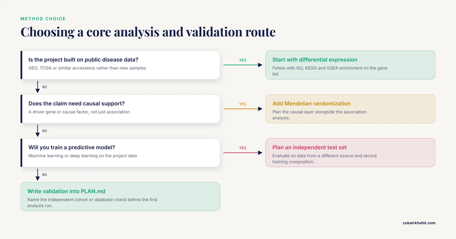
The planning phase is where method choices belong. This table maps common project types to a defensible core design.
| Project type | Core analysis | Feature selection option | Validation approach | Example in literature |
|---|---|---|---|---|
| Public-data disease mechanism | Differential expression, enrichment (GO, KEGG, GSEA) | LASSO, SVM-RFE, random forest | Independent cohort plus database expression check | Network toxicology in HCC [2] |
| Toxic exposure mechanism | Target-disease intersection, immune microenvironment | Machine learning hub gene detection | Mendelian randomization for causal support | Nicotine and spontaneous abortion [3] |
| Neurodegeneration multi-omics | Integrative GEO analysis, single-cell subclustering | LASSO, random forest, SVM-RFE | MR plus scRNA-seq transcription factor analysis | Huntington disease targets [5] |
| Clinical risk prediction | Supervised classification with held-out test set | Elastic Net, XGBoost with feature importance | Error analysis on held-out patients | Autoinflammatory disease HPO validation [6] |
| Severity prediction from multi-domain data | Integrated clinical, genomic, and epidemiological features | Five-model comparison, best model selected | Independent temporal validation cohort, SHAP interpretation | COVID-19 severity in Jiangsu [7] |
| Causal factor discovery | Causal graph construction on clinical data | Ensemble Random Forest weighting for search ordering | Synthetic and empirical benchmark comparison | Adaptive causal discovery for type 2 diabetes [8] |
Two patterns across these studies are worth internalizing. First, no single algorithm carries a result. Multi-method agreement, such as three feature selectors converging, or a model comparison across five algorithms with an independent validation cohort, is the norm in publishable work [3][7]. Second, interpretation matters as much as prediction. SHAP-based interpretation identified age as the dominant predictor of COVID-19 severity, ahead of viral features [7], and SHAP-guided marker selection was used to propose concrete genome designs in cotton breeding [9]. Plan the interpretability layer when you plan the model, not after.
A caution on training data that belongs in every deep learning plan. A systematic cross-training analysis of RNA 3D structure quality predictors found that the effect of the training dataset was large and model-dependent, with some predictors performing better on nonnative training sets than on their own [10]. The practical consequence for your plan: if you train any model, record the exact training set composition, and evaluate on data drawn from a genuinely different source than the training data. Cross-dataset generalization is not guaranteed by good benchmark scores on the home dataset.
Data Sharing, Ethics, and Governance Planning
Plan data governance when you write the plan, not at submission time. A systematic review of collaborative human genomic research in low and middle income countries documented that funding agencies increasingly require researchers to include data sharing plans in new proposals unless there are strong and clearly justified reasons to withhold data, and that sharing raises significant ethical, legal, and social concerns around consent, governance, and community context [1]. Translate that into three template fields:
- Deposition target. Which repository receives the data at publication, for example GEO for expression data, and under which accession embargo.
- Consent and restrictions. Whether the consent covering the samples permits controlled-access or public release, and who holds the keys during any embargo period.
- Human-readout risk. Whether the data could be re-identified, which determines whether the repository should be public or controlled access.
If your project touches human genomic data, write these three answers in PLAN.md before analysis begins, because they affect how you store and name files from day one.
Communicating the Plan and the Results
A project plan is also a communication instrument. Multidisciplinary teams fail at the handoff between analysis and decision-making more often than at the analysis itself. A scoping review of data visualization in clinical oncology tumor boards found that interdisciplinary conferences depend on customized tools that integrate, link, and visualize data from every profession involved, and that visualization choice shapes how the team uses molecular and clinical information [11]. Your equivalent deliverable is the report. Build it as a rendered document, for example an RMarkdown or Quarto file, so that every figure in it is generated by code that a collaborator can read.
Structure the final report around the plan fields: the question, the data, the method, the primary result, the validation, and the limitations. A reviewer or tumor board member should never have to ask how a number was produced.
If your project involves machine learning predictions used by clinicians, plan the honesty layer too. A systematic review of artificial intelligence for thymic epithelial tumors found that models using combined clinical and radiomics data tended to perform better than single-data-type models, and that some AI models outperformed physicians on certain tasks, but the review also cataloged the breadth of model types and their varied implications for rare-disease diagnosis and prognosis [12]. State in the plan who consumes the prediction and what happens when the model is wrong.
Planning in Teaching and Learning Contexts
If you are building a project to learn bioinformatics, the same template applies, scaled down. Course-based undergraduate research experiences have quantified what students gain from structured projects. In a biochemistry laboratory CURE spanning five semesters and more than 300 students, over 90 percent of students reported increased knowledge, experience, and confidence in the anticipated learning outcomes, 96 percent reported an increase in bioinformatic techniques, and 85 percent reported an increase in questions about wet-lab experiments, with no significant difference between hybrid and in-person course modalities [13]. The lesson for self-learners: the gains came from doing a bounded, planned project with defined deliverables, not from open-ended exploration. Pick one small question, one public dataset, and one deliverable, and apply the twelve-field template. A structured bioinformatics course followed by one complete planned project teaches more than three unstructured tutorials.
Common Mistakes and Limitations
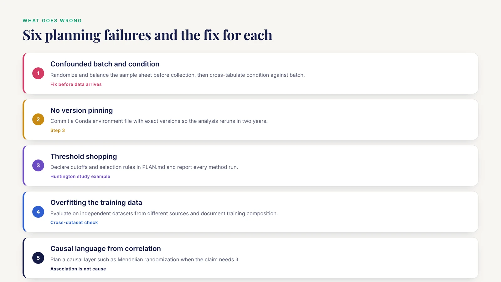
These are the failures I see most often, with the fix for each.
- Confounded design. Batch or sequencing lane perfectly aligned with the condition of interest. Fix: randomize and balance the sample sheet before data collection, and verify with a cross-tabulation of condition against batch [4].
- No version pinning. Tools installed ad hoc, so the analysis cannot be rerun. Fix: Conda environment file with exact versions committed to Git, as shown in Step 3.
- Threshold shopping. Running the analysis, then choosing the p-value cutoff or the feature selection method that gives the nicest figure. Fix: declare thresholds and method-selection rules in PLAN.md, and report all methods run, the way the Huntington study reported all three selectors and their intersection.
- Overfitting training data. Deep learning or ML performance reported on data too similar to the training set. Fix: evaluate on independent datasets from different sources, and document training data composition explicitly [10].
- Causal language from correlational data. Calling a differentially expressed gene a driver without causal evidence. Fix: plan a causal layer if the claim needs it, for example Mendelian randomization, which is how two studies above moved from association toward causal support [3][5].
- Metadata as free text. Columns like "treatment" filled inconsistently across sites. Fix: a fixed vocabulary per column, validated with a short script, in the sample sheet.
- Validation as an afterthought. Planning the confirmation step only after seeing the primary result. Fix: field 9 of the template is filled in before the first analysis run.
- Unplanned data sharing. Depositing or withholding data without checking consent terms and funder requirements. Fix: write the three governance fields into the plan at the start.
The template limits itself: a written plan does not guarantee a correct result. It guarantees that you can find out where the result went wrong, and that another person can rerun your path. Individual biological conclusions still require domain expertise and, in clinical contexts, professional judgment.
Frequently Asked Questions
What should a bioinformatics project planning template include?
Twelve fields: project ID, biological question, hypothesis, data sources with accession numbers, sample size and design, a fixed metadata schema, the primary analysis, secondary analyses with predeclared cutoffs, a validation plan, deliverables, environment and reproducibility details, and risks with decision points. Fill all twelve before running any analysis.
How do I plan a bioinformatics project from scratch if I have never done one?
Write the twelve-field plan for one small public dataset, scaffold the directory and environment exactly as shown in Steps 1 through 3 of this article, and run a two-rule Snakemake pipeline end to end on test data before the real data arrives. A complete planned project on six samples teaches the full workflow.
Where can I find a free bioinformatics project planning template?
The twelve-field table in the section "The Bioinformatics Project Planning Template Format" is free to copy, and the PLAN.md file created in this walkthrough is that template in plain text form. No special software is needed to use it.
How much data do I need before starting an analysis?
Enough samples to support your primary comparison without confounding, which means design balance matters more than raw count. Check your sample sheet for balanced condition and batch counts before analysis, and plan the statistical model around the design you actually have.
How do I keep a bioinformatics project reproducible?
Pin tool versions in a Conda environment file, keep raw data read-only, regenerate all results from code through a workflow manager such as Snakemake, commit the plan, code, and configuration to Git, and record the exact training data composition for any model you fit.
Do I need a bioinformatics course to plan a project?
No, but structured instruction accelerates it. Course-based research experiences show that students completing planned projects report large gains in bioinformatic technique and confidence, so a course or structured project is the efficient path even though self-teaching works.
How do I plan for data sharing and ethics?
Write the deposition repository, the consent restrictions on release, and the re-identification risk into the plan before analysis starts, since funding agencies increasingly require explicit data sharing plans and sharing raises ethical, legal, and social questions that affect how you store data from day one.
How long does a bioinformatics project take?
It depends on data volume, compute availability, and validation depth, so plan with milestones rather than a single deadline. Typical milestones are environment setup, QC sign-off, primary analysis complete, validation complete, and report delivered, each written into the plan with an owner and a target date.
Sources
- Context of data sharing practices in collaborative human genomic research in low and middle income countries: A systematic review.
- Deciphering the mechanism of aristolochic acid I-driven hepatocellular carcinoma through integrated network toxicology and bioinformatics.
- Identification of key molecular targets in nicotine-induced spontaneous abortion through network toxicology and multi-omics integration.
- Automating Large-Scale Experiment Scheduling and Planning with the WorkListGenerator.
- Bioinformatics Analysis to Reveal Potential Targets of Huntington's Disease.
- Machine learning-based validation of Human Phenotype Ontology (HPO) terms for systemic autoinflammatory diseases using the Eurofever Registry: the ODINO project.
- A population-based retrospective machine learning study of COVID-19 severity using integrated clinical and viral genomic data in Jiangsu Province, China.
- Adaptive causal discovery with ordering-based reinforcement learning-approach for type 2 diabetes mellitus risk factors.
- A predictive approach to genome design for multi-trait improvement and environmental adaptability via machine learning.
- Impact of training data on deep learning-based RNA 3D structure quality assessment.
- Data Visualization Support for Interdisciplinary Team Treatment Planning in Clinical Oncology: Scoping Review.
- Artificial intelligence for diagnosis and prognosis of thymic epithelial tumors: a systematic review.
- Analysis of Perceived Student Learning Gains in a Biochemistry Lab Course-Based Undergraduate Research Experience.