Bioinformatics Data Lifecycle: Transitioning Between Stages
By Dr. Zubair Khalid, DVM, MS, PhD ·

By the end of this article you will be able to map your project onto the standard bioinformatics data lifecycle workflow, define hard checkpoints for transitioning bioinformatics data between lifecycle stages, run the validation commands that make each handoff safe, and choose storage and deposition options that keep your data usable years later. Everything is written from the perspective of a working bench bioinformatician or core facility analyst who has to move real files, not diagrams.
You will need a Linux or macOS shell, Python 3 with the Conda package manager (Miniforge or Miniconda), the Snakemake workflow manager, and about 3 to 5 times the size of your raw dataset in free disk space for a typical sequencing project. A text editor, a version control repository for scripts, and a spreadsheet program for the sample sheet round out the toolkit.
What the Bioinformatics Data Lifecycle Actually Covers
Most working definitions of the bioinformatics data lifecycle break into six stages:
- Planning and acquisition. You define the biological question, the sample metadata schema, and how samples and files will be tracked from the freezer to the sequencer.
- Ingest and validation. Raw data arrive, you verify integrity with checksums, confirm sample identities, and run first-pass quality control.
- Processing and analysis. Reads are trimmed, filtered, assembled, aligned, or quantified according to a scripted, versioned workflow.
- Result curation. Outputs are summarized, quality assessed a second time at the analysis level, and linked back to sample metadata.
- Storage, sharing, and deposition. Data move to durable storage and, where required, to public archives with standardized metadata.
- Reuse and long-term stewardship. Published or archived data get retrieved, transformed, and reanalyzed by you or by others.
Published platforms in the life sciences describe the same shape. The Barcode of Life Data System explicitly supports acquisition, storage, validation, analysis, and dataset publication within one collaboration model [1]. BioStudies at EMBL-EBI organizes datasets across data acquisition during collaborative projects, deposition at manuscript submission, and post-publication data packages [2]. The lesson from both is that the lifecycle is not a straight line you walk once. Data loop backward: a validation failure at stage 2 sends you back to stage 1 metadata. A reviewer request at stage 5 sends you back to stage 3 reprocessing. The transitions are where projects succeed or fail.
Why do transitions deserve their own attention? Because each stage has different owners, different file formats, different storage media, and different failure modes. Raw FASTQ files belong on cheap, large, protected storage. Processed count matrices belong next to the code that made them. The moment data cross a stage boundary without a checkpoint, you lose the ability to answer two questions later: where did this file come from, and can I regenerate it?
Stage 1: Planning and Acquisition
The single highest-leverage decision in bioinformatics data management happens before any data exist: the design of the sample metadata record. Laboratory information management systems built for high-throughput facilities track samples and associated metadata from the beginning to the end of an experiment, including processing and archiving, because retrofitting metadata after the fact rarely works [3].
Build the sample sheet first
Create a sample sheet as a plain CSV before samples ship to the sequencer. A workable minimal schema for a sequencing project looks like this:
sample_id,condition,replicate,tissue,collection_date,operator,library_type,lane
S001,control,1,liver,2026-03-14,JGM,RNA-seq,1
S002,control,2,liver,2026-03-14,JGM,RNA-seq,1
S003,treated,1,liver,2026-03-15,JGM,RNA-seq,1
S004,treated,2,liver,2026-03-15,JGM,RNA-seq,1
Rules that pay for themselves:
sample_idmust be unique, stable, and never reused, even if a sample fails.- Dates use ISO format (YYYY-MM-DD) so they sort correctly in every language.
- Every column that an analysis will ever stratify on (condition, tissue, batch) gets a column now. Adding columns later requires guessing.
- Keep one canonical copy of the sample sheet in version control. Copies floating in email are a known source of sample swaps.
If your project spans multiple laboratories or a core facility, a LIMS with defined user groups, privileges, and project-level metadata storage replaces the spreadsheet. Systems designed for this purpose carry quote, project, and node management across single and multisite networks, which matters when the person generating data is not the person analyzing it [3].
Decide the metadata standard now
If your data will eventually be deposited, check the metadata requirements of the target archive during planning, not at submission time. Platforms such as BioStudies let communities define and implement metadata guidelines tailored to specific data types, and they organize submitted datasets into collections [2]. Harmonization efforts in biological imaging make the same argument from the AI side: shared data only become computationally ready when they carry standardized, context-rich annotation and interoperable formats from the start [4]. Writing your sample sheet in the target standard's vocabulary at stage 1 removes an entire category of painful conversion at stage 5.
Stage 2: Ingest and Validation
Data leave the sequencer and arrive on your storage. This transition has three non-negotiable checkpoints: integrity, identity, and quality.
Checkpoint 1: Verify file integrity
Sequencing providers deliver a manifest with MD5 or SHA-256 checksums. Verify before you do anything else:
# Run in the directory containing the delivered FASTQ files
sha256sum *.fastq.gz > sha256.local.txt
cat sha256.local.txt
Expected output looks like this:
a3f8c1e9b2d4...  S001_R1.fastq.gz
77b2e0aa41cf...  S001_R2.fastq.gz
9c41d8f7e6b5...  S002_R1.fastq.gz
Compare against the provider manifest:
diff <(sort sha256.local.txt) <(sort sha256.provider.txt)If diff prints nothing, the files transferred intact. If it prints a mismatched line, redownload that file before proceeding. Run the same verification again whenever you copy raw data to a second location, such as an archive volume or cloud bucket. Never trust a copy without a checksum.
Checkpoint 2: Confirm sample identity
Read the first four lines of each FASTQ file and confirm the read name prefix matches the expected sample barcode or index:
zcat S001_R1.fastq.gz | head -n 4Expected output:
@A00552:123:HTKWLDSX7:1:1101:2464:1000 1:N:0:ATCACG
GATCGGAAGAGCACACGTCTGAACTCCAGTCA
+ \\
AJJJJJJJJJJJJJJJJJJJJJJJJJJAJJJJ
The 1:N:0:ATCACG tail carries the index sequence. A mismatch between the index in the file and the index in your sample sheet is the classic sign of a swapped or skipped sample. Catching it here costs minutes. Catching it after differential analysis costs the project.
Checkpoint 3: First-pass quality control
Run FastQC on every file and aggregate with MultiQC:
mamba create -n qc -c bioconda fastqc multiqc
conda activate qc
fastqc *.fastq.gz -t 8 -o fastqc_raw/
multiqc fastqc_raw/ -o multiqc_raw/
MultiQC prints a summary like:
[  4/4 ] fastqc: S004_R2      ██████████████████████ 100%
MultiQC report generated: multiqc_raw/multiqc_report.html
Open the HTML report and check per-base sequence quality (Phred scores above 30 across most of the read), adapter content, and per-sequence GC content. Record the decisions you make here (for example, trim the first 12 bases, discard reads shorter than 50) in a text file inside the project directory. Quality assessment at this stage is not optional. The machine learning lifecycle literature emphasizes rigorous quality assessment during data preparation as a precondition for everything downstream [5], and the same principle holds for classical statistics.
At this point raw data are locked. Copy them to at least two physical locations, apply checksums to the copies, and treat them as read-only. Everything after this point should be regenerable from the locked raw files plus your code.
Stage 3: Processing and Analysis
The transition from validated raw data to processed results should be executed by a workflow manager, never by hand-typed commands scattered across a shell history. Workflow managers exist precisely to assist in the design of complex, long-running, data-intensive experiments composed of many processing tasks [6], and to make every intermediate file traceable to the command and parameters that produced it.
Encode the workflow in Snakemake
Create a Snakefile in the project root:
SAMPLES = ["S001", "S002", "S003", "S004"]

rule all:
    input:
        expand("results/{sample}/trimmed_R1.fastq.gz", sample=SAMPLES),
        "qc/multiqc_report.html"

rule trim:
    input:
        r1="raw/{sample}_R1.fastq.gz",
        r2="raw/{sample}_R2.fastq.gz"
    output:
        r1="results/{sample}/trimmed_R1.fastq.gz",
        r2="results/{sample}/trimmed_R2.fastq.gz"
    log:
        "logs/trim/{sample}.log"
    shell:
        "cutadapt -a AGATCGGAAGAGC -A AGATCGGAAGAGC "
        "-m 50 -q 20 "
        "{input.r1} {input.r2} "
        "-o {output.r1} -p {output.r2} > {log} 2>&1"

rule multiqc:
    input:
        expand("results/{sample}/trimmed_R1.fastq.gz", sample=SAMPLES)
    output:
        "qc/multiqc_report.html"
    shell:
        "multiqc results/ -o qc/"
Test the plan before running anything:
snakemake --cores 8 --dry-runExpected output:
Building DAG of jobs...
Job stats:
job       count
------    -----
all           1
multiqc       1
trim          4
total         6

This was a dry-run.
Then execute:
snakemake --cores 8 --use-condaExplain the parameters to yourself in the project README, because future you is the most common reader:
-cores 8reserves eight threads for the whole run. Snakemake distributes them across rules.-use-condamakes each rule resolve its software into an isolated environment defined in anenvs/YAML file, so the workflow carries its own dependency list.-m 50in cutadapt discards reads shorter than 50 bases after trimming.-q 20trims low-quality ends below Phred 20, which corresponds to a 1 in 100 probability of base-call error.
Automated pipelines demonstrate how much of this chain can be standardized. Sphae, a Snakemake-based pipeline for phage therapy screening, integrates quality control, assembly, genome assessment, and annotation, and automates detection of markers such as virulence factors, antimicrobial resistance genes, and lysogeny indicators, producing an assessment in under ten minutes per phage [7]. Benchmarking on 65 phage sequences showed 28 candidates with therapeutic potential, 8 failures during assembly attributable to low sequencing depth, 22 samples carrying prophage or virulence markers, and 23 samples containing multiple phage genomes per sample [7]. That failure breakdown is instructive for any lifecycle: failures cluster at predictable transitions (assembly depth, mixed samples), and a well-built workflow surfaces them as named categories rather than silent bad output.
Web-integrated platforms compress the same lifecycle for users who cannot maintain a cluster. LoadExp+ ties RNA-seq, bisulfite-seq, ChIP-seq, and variant workflows into the CoGe comparative genomics platform, with all analyses available for visualization and export to external data management platforms [8]. Cloud platforms such as Wekemo Bioincloud offer dozens of standardized multi-omics workflows with AI-assisted parameter selection, reducing the technical barrier for groups without dedicated informaticists [9]. For structured tutorial-style coverage of an entire analytical chain in one language, the R-based lipidomics roadmap organizes the lifecycle from raw acquisition through preprocessing, annotation, statistical modeling, and functional interpretation with named packages at each step [10].
Whichever execution environment you choose, the transition into stage 3 is only complete when three things are true: the workflow runs from raw data to results with one command, every parameter is recorded in versioned files, and the software versions are pinned.
Validate at the analysis level
Quality control repeats at the processed stage, and it looks different. For count-based assays, inspect library sizes, mapping rates, and sample clustering:
library(DESeq2)
dds <- DESeqDataSetFromMatrix(countData = counts,
                              colData = meta,
                              design = ~ condition)
vsd <- vst(dds)
plotPCA(vsd, intgroup = "condition")
If replicates cluster by collection date instead of condition, you have a batch effect, and no amount of downstream statistics will rescue it. That discovery sends you back to the design table, which is exactly the kind of backward transition a lifecycle framework is supposed to anticipate. Methodological guidance in quantitative omics fields stresses anticipating statistical assumptions and reproducibility constraints at the workflow design stage rather than after results appear [10].
The Transition Points: A Checkpoint Table
Every stage handoff should pass a gate. The table below summarizes the minimum checkpoint for each transition in a bioinformatics data lifecycle workflow, the command or artifact that proves the gate passed, and what to write down.
| Transition | Gate condition | Proof artifact | Record in |
|---|---|---|---|
| Acquisition to ingest | Files match provider checksums | sha256sum diff with no output | Project log |
| Ingest to raw archive | Identity confirmed, QC reviewed, two copies exist | Sample sheet crosscheck, MultiQC report, two checksum files | README and LIMS entry |
| Raw archive to processing | Workflow dry-runs clean, software pinned | snakemake, dry-run output, environment YAML files | Git tag |
| Processing to analysis | Mapping or assembly metrics within expectations | MultiQC on processed data, alignment summary table | Notebook entry |
| Analysis to curation | Results reproduce from a clean checkout | Fresh snakemake, cores 8, use-conda run on a collaborator machine | Git tag plus results hash |
| Curation to deposition | Metadata matches archive standard, embargo set | Archive validation report | Submission record |
| Deposition to reuse | Accession resolves, files download, checksums match | Test download with sha256sum | Publication data availability statement |
Two of these gates deserve elaboration because they fail most often.
The raw-to-processing gate. The most common failure is silent parameter drift: someone reruns trimming with -q 15 instead of -q 20 and does not record it. The defense is to never run processing commands interactively on data destined for publication. If a command is not in the Snakefile, it did not happen.
The curation-to-deposition gate. Archives validate structure, not biology. A file can pass upload validation while containing the wrong sample in the wrong column. Before deposition, recompute a random sample of derived values from the raw data and compare against the deposited tables. For imaging and other multidimensional data, harmonization guidance explicitly calls for standardized annotation and quality controls as the condition for data becoming computationally ready for reuse [4], and the same standard applies to genomics.
Stage 4: Storage Architecture for Genomics Data
Genomics data storage decisions follow file temperature. Hot data (active analysis) live on fast local scratch. Warm data (recently completed projects) live on a shared filesystem. Cold data (raw files awaiting reuse) live on cheap, redundant, geographically separated storage.
A practical layout for one project:
project_phageR/
├── raw/                  # read-only, checksummed, 2 copies minimum
│   ├── S001_R1.fastq.gz
│   └── sha256.local.txt
├── results/              # regenerable, may be deleted and rebuilt
├── qc/                   # reports kept permanently
├── envs/                 # conda environment YAML files
├── logs/
├── Snakefile             # in git
├── samplesheet.csv       # in git
└── README.md             # decisions, in git
The raw directory is the only irreplaceable content, so it gets the storage budget. Raw paired-end Illumina runs run from roughly 1 to 40 GB per sample depending on read length and depth, so a 96-sample project can hold several terabytes of raw data alone. Budget raw capacity first, then add scratch space of at least twice the raw volume for intermediates.
Regenerable outputs do not need backup, they need reproducibility. If you can rebuild results/ from raw/ plus a git tag, you do not archive intermediates. That distinction cuts storage costs sharply and is one of the most useful bioinformatics data lifecycle workflow tips for groups hitting quota limits.
Integrated platforms blur these boundaries productively. CoGe's LoadExp+ keeps analyses attached to the genomes they ran against and exports results to CyVerse's data management and analysis platforms for longer-term handling [8]. BOLDconnectR provides authenticated programmatic access to a centralized workbench, returning records in a standard data model so downstream pipelines do not depend on screen scraping [1]. The pattern in both cases is the same: move data between systems through APIs with defined data models, not through ad hoc file exports, because the API path records provenance and the export path does not.
Stage 5: Publication, Sharing, and Deposition
The transition to public sharing has its own mechanics. BioStudies accepts descriptions of studies that do not fit specialized archives, links them to data held internally or externally, and supports the full path from project-internal sharing through deposition at manuscript submission to post-publication data packages [2]. The platform has also served projects migrating from legacy data infrastructures, which is a reminder that deposition systems themselves have lifecycles, and choosing one with sustainable archival commitments protects your accession links from rotting.
A deposition checklist that survives review:
- Freeze the analysis. Tag the git repository (for example,
git tag v1.0-publication), record the commit hash in the README, and run the workflow one final time from a clean checkout. - Export data in community formats. Conversion failures at submission time are the most common cause of delayed deposits.
- Map sample sheet columns to the archive's metadata schema. Reusing the vocabulary you chose in stage 1 makes this a lookup rather than a translation.
- Generate checksums for every deposited file and include the checksum file itself.
- Record the accession number in the manuscript data availability statement and, ideally, in the README of the code repository.
For data feeding machine learning, the deposition question extends to model artifacts. The clinical microbiology ML lifecycle literature treats data preparation, model development, evaluation, and deployment as one continuous chain and warns that evaluation challenges such as class imbalance, generalization, and robustness surface at deployment if they were not addressed during development [5]. Deposit the training data partition definitions alongside the data, or the model cannot be honestly re-evaluated.
Stage 6: Governance, Security, and Production Deployment
Once a pipeline leaves the one-project, one-analyst world and becomes infrastructure that others depend on, the lifecycle gains governance requirements that individual projects can ignore.
Security and ethics constraints belong in the workflow design itself. Early work on semantically aware bioinformatics workflow environments emphasized secure enactment of experiments and built reasoning support for the security and ethical requirements of data-processing scenarios [6]. In practice this means access control on human-derived data, audit logs on who ran what, and explicit handling rules for identifiable information before the first job executes, not after an incident.
Real-world clinical deployments illustrate what production stewardship looks like. The A-GPS asthma decision support system was built on a disease-agnostic platform with an API-first backbone of reusable services, integrating multiple data sources into a decision-relevant summary at the point of care, with an accompanying lifecycle governance framework covering development, evaluation, and implementation [11]. The transferable lesson for bioinformatics teams is the API-first structure: services that expose data through stable interfaces survive reorganization far better than file shares that everyone accesses by personal scripts.
Monitoring closes the loop. A deployed model or pipeline degrades as inputs drift, and the ML lifecycle framework treats post-deployment evaluation as part of the lifecycle rather than an endpoint [5]. Schedule a periodic revalidation: rerun the workflow's QC stages on a fixed reference input and compare against stored baseline metrics. If metrics move without a code change, your environment drifted, and you want to know that before a collaborator finds it.
Practical Tips for Transitioning Between Stages
These are the habits that separate lifecycle workflows that survive a funding cycle from those that collapse at the first personnel change.
- Freeze raw data with chmod. After checksums pass,
chmod -R a-w raw/on the project directory. The typo that deletes raw data is made by senior people under deadline pressure. - Tag every stage transition in git. A tag at raw-data-lock, a tag at analysis-freeze, a tag at deposition. Tags are cheap and answer the "which version produced figure 3" question instantly.
- Write the run log as the workflow runs. Snakemake's
-reportflag generates a self-contained HTML report of the entire execution, including software versions and file provenance. Attach it to the project record at every stage gate. - Keep one canonical sample sheet. All analyses read from it. Nobody edits copies.
- Test the restoration path, not just the backup. A backup you have never restored from is a hope, not a backup. Restore one raw file from each storage tier annually and verify its checksum.
- Automate the boring gates. A five-line shell script that verifies checksums and diffs the sample sheet against the raw file list turns the ingest checkpoint from a chore into a preflight check nobody skips.
- Design transitions for your successor. Assume the person executing the reuse stage in year three is not you. Directory names, README text, and metadata vocabulary should be self-explanatory without oral tradition.
Common Mistakes and Limitations
These are the failures seen repeatedly when projects transition between lifecycle stages, with the specific mechanism of each.
Treating QC as a stage rather than a property. Quality control happens at ingest, after processing, after statistical modeling, and before deposition. Projects that run FastQC once and move on discover adapter contamination in their assembled contigs. Build a QC rule into every stage of the workflow.
Storing intermediates instead of regenerating them. Archiving every BAM and bigWig file "just in case" fills storage within months and creates dozens of unversioned file variants. If a file is deterministically regenerable from raw data plus versioned code, delete it on a schedule and keep the recipe.
Metadata drift. The sample sheet says treated, the LIMS says Treated, the count matrix column says trt. String-matching across these variants consumes days and introduces silent errors. Enforce a controlled vocabulary from stage 1 and validate the sample sheet with a script at every gate.
Checksums on write, never on read. Teams verify checksums when data arrive and then never again. Storage decays. Verify checksums at every copy operation and during archival reads, not just at delivery.
Interactive analysis on publication-bound data. An analyst opens a REPL, filters a table by eye, saves an overwritten copy, and the workflow no longer reproduces the published result. The fix is procedural: publication-bound outputs come only from the workflow, and exploratory work happens on copies in a separate directory.
Confusing backup with versioning. A nightly backup of a directory that contains three contradictory versions of results.csv backs up confusion. Versioning (git for code and metadata, immutable timestamps for outputs) and backup solve different problems and you need both.
Ignoring the reuse stage until someone emails you. Data deposited with missing unit annotations, unspecified genome builds, or undeclared missingness generate emails for years. Run the retrieval test yourself: download your own deposit through its public API, recompute one result, and confirm it matches. Programmatic retrieval through defined data models, as supported by packages built for this purpose [1], is the standard your deposit should meet.
A final limitation applies to everything above: the specific thresholds, tools, and storage budgets are starting points calibrated for typical sequencing projects. Individual projects with unusual data types, regulated human data, or clinical deployment obligations need their own governance review, and no generic workflow article substitutes for institutional policy on those cases.
Frequently Asked Questions
What are the stages of the bioinformatics data lifecycle?
The commonly used stages are planning and acquisition, ingest and validation, processing and analysis, result curation, storage and deposition, and reuse or long-term stewardship. Different platforms name them differently, but published systems from repositories to LIMS implementations all cover the same arc from sample creation through publication to reuse.
Why do data transitions between stages cause the most problems?
Each stage has different owners, formats, and storage systems, so information that is implicit in one stage (which sample this file came from, which parameters produced it) becomes lost at the boundary. Checkpoints with checksums, sample sheet crosschecks, and versioned code restore that information at every handoff.
What commands should I run when raw sequencing data arrive?
Run sha256sum or md5sum on every file and diff the output against the provider manifest, inspect the first lines of each FASTQ for index sequence identity, then run FastQC and aggregate with MultiQC. Only after all three checks pass should raw files be copied to read-only archive storage with checksums recorded for each copy.
How much storage do I need for a genomics project?
Plan for raw data plus two to four times the raw volume in scratch space for intermediates during processing. Raw paired-end sequencing files range from roughly 1 to 40 GB per sample depending on read length and depth, so a 96-sample project can easily require multiple terabytes for raw data alone. Regenerable intermediates need scratch capacity, not backup.
Should I back up intermediate files like BAM files?
No, if they are deterministically regenerable from raw data and versioned code. Store the recipe (the workflow, software environments, and parameters) under version control and regenerate intermediates on demand. Back up only the raw data and the small files that are not regenerable, such as QC reports and the sample sheet.
How do I prepare data for public deposition?
Freeze the analysis with a git tag, convert files to community-accepted formats, map your metadata to the target archive's schema, generate checksums for all deposited files, and record the accession in the manuscript. Depositing the metadata vocabulary you designed at the start of the project makes this step a lookup rather than a rebuild.
What is the difference between a workflow manager and a LIMS?
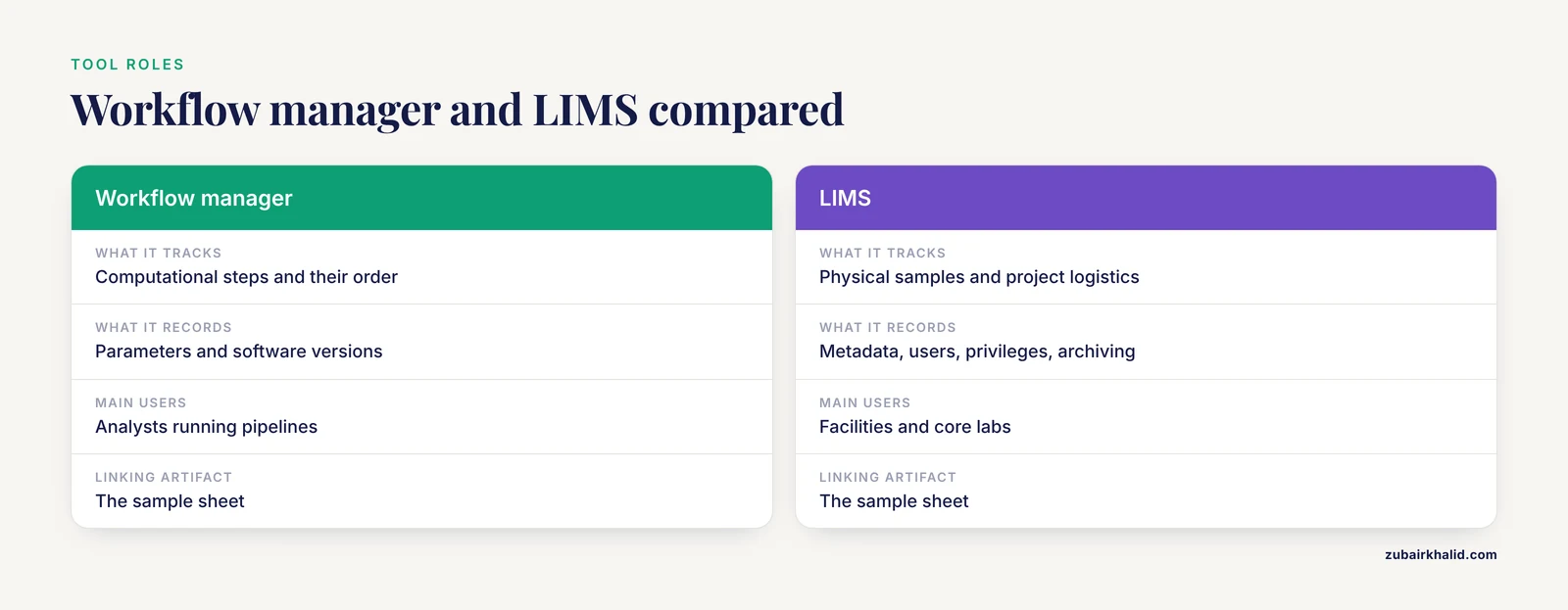
A workflow manager such as Snakemake executes computational steps in the right order with recorded parameters and software versions. A LIMS tracks physical samples, metadata, users, and project logistics from collection through archiving. Larger facilities need both, and the sample sheet is usually the artifact that links them.
How often should I validate stored data after archiving?
Verify checksums every time data are copied between systems, and schedule at least an annual read test on archived copies where you restore and checksum a sample of files. Storage media and cloud objects decay or drift quietly, and an unverified archive is an assumption rather than a backup.
Sources
- BOLDconnectR: An R package for streamlined retrieval, transformation, and analysis of DNA barcode data on BOLD.
- BioStudies Database: A Platform for Life Sciences Study Data Dissemination.
- MASTR-MS: a web-based collaborative laboratory information management system (LIMS) for metabolomics.
- Harmonizing the Generation and Pre-publication Stewardship of FAIR bioimage data.
- An introduction to the machine learning lifecycle for clinical microbiology.
- A semantically aware platform for the authoring and secure enactment of bioinformatics workflows.
- phage therapy candidates from Sphae: An automated toolkit for predicting sequencing data.
- CoGe LoadExp+: A web-based suite that integrates next-generation sequencing data analysis workflows and visualization.
- Wekemo Bioincloud 2026: An AI-enabled platform for standardized multi-omics data analyses.
- A Structured Computational Roadmap for Lipidomics in R: Reproducible Workflows from Raw Data to Functional Insight.
- A lifecycle governance and learning health system framework for trustworthy, generalizable, and sustainable human-ai partnership in clinical practice: Lessons from the asthma-guidance and prediction system (A-GPS).