Best R Packages for Single-Cell RNA-seq Analysis

By Dr. Zubair Khalid, DVM, MS, PhD · 2026-11-11

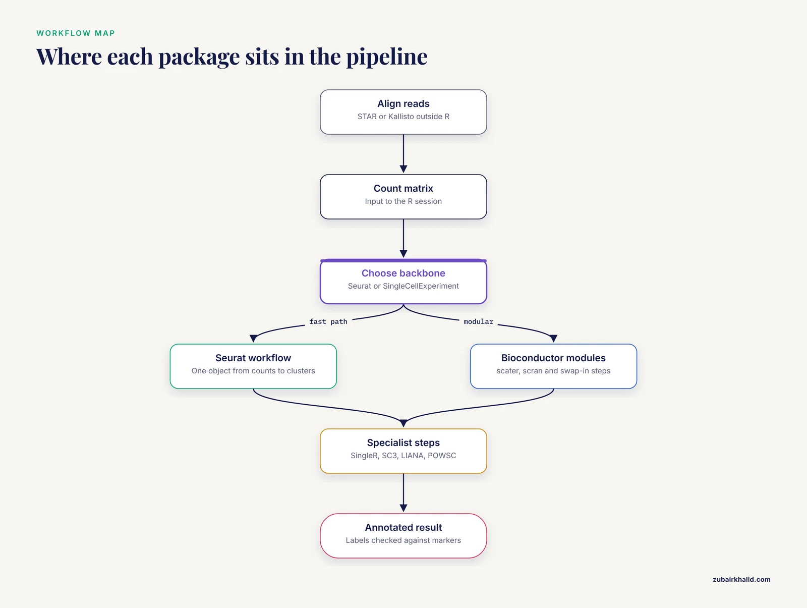
The single most important difference between the best R packages for single-cell RNA-seq analysis is scope: Seurat and the Bioconductor SingleCellExperiment ecosystem are general-purpose workflow frameworks that handle a full analysis end to end, while packages like SingleR, SC3, LIANA, and POWSC are specialists that outperform general tools at one specific task. The practical rule of thumb is simple: pick one framework (Seurat or Bioconductor) for the backbone of your workflow, then bring in benchmark-winning specialist packages for the steps where accuracy matters most, such as cell type annotation and clustering.

This guide walks through those options stage by stage, states the pros and cons of each package, cites the benchmark studies that compared them, and ends with worked scenarios and the mistakes analysts make most often.

Why R Dominates Single-Cell RNA-seq Workflows

R for bioinformatics has become the default language for single-cell work for three reasons. First, the two most widely used analysis frameworks, Seurat and the Bioconductor ecosystem, are written in R and expose every step of a standard workflow as reusable functions. Second, CRAN and Bioconductor host hundreds of peer-reviewed method packages, so new algorithms arrive as installable R libraries rather than standalone programs. Third, R's plotting system (ggplot2) produces publication-quality figures directly from analysis objects, which keeps visualization and computation in one script.

Bioconductor deserves special mention. It is a curated, open-source repository of R packages for genomic data analysis with strict standards for documentation and testing. Every Bioconductor package ships a vignette, a worked example document that functions as a bioconductor tutorial, and packages such as scater, scran, and SingleCellExperiment have vignettes detailed enough to serve as complete analysis walkthroughs. If you are learning the field, working through one Seurat vignette and one Bioconductor vignette on the same dataset is the fastest way to understand where the two ecosystems differ.

One boundary worth stating up front: R packages do not handle the raw alignment step of droplet data well. That stage is dominated by command-line tools such as Cell Ranger, STAR, and Kallisto, which are covered later in this article because benchmark data on them directly affects what lands in your R session.

The Two Frameworks: Seurat and Bioconductor

Flowchart from command-line alignment through Seurat or Bioconductor backbone, then specialist steps for annotation, integration and communication.

Seurat

Seurat is the most widely used end-to-end R framework for single-cell RNA-seq analysis. A typical Seurat script creates a Seurat object from a count matrix, filters cells and genes, normalizes, identifies highly variable genes, runs PCA, builds a shared nearest neighbor graph, clusters, and visualizes with UMAP, all in roughly twenty lines of code.

Pros:

Complete workflow from count matrix to annotated clusters in a single object model
Excellent documentation and a large user community, so almost any error message has been solved publicly
Benchmark evidence supports it at two separate steps. In a comparison of ten cell type annotation packages, Seurat performed well overall and was the best at annotating major cell types [1]. In a systematic evaluation of twelve clustering algorithms across nine datasets and three simulations, Seurat and SC3 showed the most favorable results [2]

Cons:

Seurat's own annotation strength depends on having reference clusters to transfer labels from, so it is not a standalone annotation solution for unfamiliar tissues
The object model is proprietary to Seurat, which complicates interoperability with Bioconductor tooling
Integration and large-dataset handling can be memory hungry

The Bioconductor SingleCellExperiment Ecosystem

The Bioconductor alternative is built around the SingleCellExperiment container, a standardized object that stores counts, transformed expression values, reduced dimensions, and metadata in one structure. Around it sit specialized packages: scater for quality control and visualization, scran for normalization, and dozens of others that all read and write the same object class.

Pros:

Modular design. You can swap any single step for a better method without touching the rest of the pipeline
Interoperability. Because every package uses SingleCellExperiment, results flow between tools without format conversion
Formal, tested infrastructure with vignettes that act as ready-made tutorials
pipeComp, an R framework developed to evaluate scRNA-seq preprocessing pipelines, benchmarked the common steps of filtering, doublet detection, normalization, feature selection, denoising, dimensionality reduction, and clustering and is itself a Bioconductor-style resource for choosing between options at each step [3]

Cons:

More setup code than Seurat for an equivalent analysis
Documentation is spread across many package vignettes rather than centralized
Beginners often struggle with which combination of modules to assemble

Side-by-Side Comparison of the Best R Packages for Single-Cell RNA-seq

The table below is the core of this article. It summarizes the package options at each workflow stage, with benchmark evidence noted where it exists.

Workflow stage	Package	Ecosystem	Pros	Cons
Full workflow backbone	Seurat	CRAN	End-to-end, best at major cell type annotation among ten benchmarked tools [1], top-tier clustering performance [2]	Closed object model, memory hungry at scale
Full workflow backbone	SingleCellExperiment, scater, scran	Bioconductor	Modular, standardized object, strong vignettes	More assembly required, steeper start
Alignment (pre-R)	STAR / STARsolo	Command line	More detected genes and higher expression values than Kallisto, better marker recovery [4]	About 4-fold slower and 7.7-fold more memory than Kallisto [4]
Alignment (pre-R)	Kallisto	Command line	Fast pseudoalignment, far lower memory use [4]	Lower gene abundance than alignment-based approaches [4]
Highly variable genes	scran modelGeneVar, Seurat	Both	Multiple options benchmarked for HVG discovery [5]	Method choice affects downstream clustering
Dimensionality reduction	UMAP	CRAN/Rcpp	Highest stability among ten benchmarked methods, good preservation of population cohesion [6]	Second highest computing cost, hyperparameter sensitive [6]
Dimensionality reduction	t-SNE	CRAN/R	Best overall accuracy among ten benchmarked methods [6]	Highest computing cost, requires tuning [6]
Clustering	Seurat graph-based clustering	CRAN	Among the most favorable in a 12-method benchmark [2]	Resolution tuning needed
Clustering	SC3	Bioconductor	Among the most favorable in the same benchmark [2]	Slower on large datasets
Clustering	Deep learning methods	Various	Reviewed as a growing class suited to sparse, high-dimensional data [7]	Immature tooling, harder to interpret
Cell annotation	Seurat label transfer	CRAN	Best at major cell types in a ten-package comparison [1]	Needs a matched reference dataset
Cell annotation	SingleR	Bioconductor	Strong performer in two independent benchmarks [1][8], robust to downsampling [8]	Reference quality drives output
Cell annotation	SingleCellNet	CRAN	Strong performer in benchmark comparisons [1]	Less widely adopted
Cell annotation	scmap, CHETAH, scID, Garnett, SCINA	Various	Available options with published evaluations [1]	Weaker overall performance than the leaders in the same benchmark [1]
Cell annotation	CP, RPC (repurposed from methylation deconvolution)	R	Performed well despite being designed for other omics data [1], robust against downsampling for CP [8]	Unfamiliar to most single-cell analysts
Batch correction	Eight methods compared via BatchBench	Various	Systematic comparison available to guide tool choice [9]	Best method is dataset dependent
Cell-cell communication	LIANA	Python/R interface	Consensus interface to seven methods and sixteen resources [10]	Predictions vary strongly by method and resource choice [10]
Power and design	POWSC	CRAN	Simulation-based power evaluation and sample size recommendation for scRNA-seq DE [11]	Focused on differential expression only

Stage 1: Alignment Before R

Everything in your R session depends on the count matrix, and the count matrix depends on how the reads were aligned. A systematic third-party comparison of STAR and Kallisto on Drop-seq, Fluidigm, and 10x Genomics data found that STAR globally produced more genes and higher gene-expression values than Kallisto, and also higher correlations of the Gini index with RNA-FISH validation results [4]. On 10x PBMC 3k data and mouse cortex single-nucleus data, STAR yielded similar or better cell-type annotation results by detecting a larger subset of known gene markers [4].

The cost is real. STAR required significantly more computation time, roughly 4-fold slower, and about 7.7-fold more memory than Kallisto [4]. In practice this means STARsolo or Cell Ranger for accuracy-critical projects with adequate compute, and Kallisto-based pipelines when speed and memory constraints dominate.

Stage 2: Quality Control, Filtering, and Doublet Detection

Quality control removes low-quality cells, empty droplets, and doublets before any downstream statistics. The packages here are scater (quality metrics and plotting), DropletUtils (empty droplet calling for droplet data), and DoubletFinder or scDblFinder for doublet removal.

Rather than guessing at which filtering and doublet tools to combine, you can rely on pipeComp, an R framework built specifically to evaluate scRNA-seq preprocessing pipelines. It handles interactions between analysis steps and uses multi-level evaluation metrics, covering filtering, doublet detection, normalization, feature selection, denoising, dimensionality reduction, and clustering on datasets with known cell identities [3]. Its practical value is that pipeline steps interact: the best doublet detector in isolation is not necessarily the best doublet detector inside your particular pipeline, and pipeComp is designed to test exactly those interactions.

A key QC insight from the alignment benchmark carries through here: filtering decisions interact with data provenance. Long-read sequencing of the same 10x cDNA allows removal of degraded cDNA contaminated by template switching oligos, artifacts that short reads cannot identify, and filtering such artifacts reduces detected expression [12]. If your data has passed through nonstandard library processing, default QC thresholds may misjudge it.

Stage 3: Normalization and Highly Variable Gene Selection

Normalization corrects for differences in sequencing depth between cells, and highly variable gene (HVG) selection decides which genes feed into dimensionality reduction and clustering. Both steps are implemented in scran and in Seurat.

An evaluation of tools for highly variable gene discovery from single-cell RNA-seq data exists specifically because this step matters so much downstream [5]. The choice of HVG method changes which genes define your clusters, and there is no single universally best tool, which is why the evaluation literature treats HVG selection as a first-class analysis decision rather than housekeeping.

Stage 4: Dimensionality Reduction

Single-cell data is high-dimensional, noisy, and sparse. Dimension reduction compresses it into a small number of dimensions for visualization and clustering.

Two benchmark studies bracket this space. A comparison of ten dimensionality reduction methods on thirty simulated and five real datasets found that t-SNE yielded the best overall performance with the highest accuracy but also the highest computing cost, while UMAP exhibited the highest stability along with moderate accuracy and the second highest computing cost [6]. The same study emphasized that users need to tune hyperparameters according to the specific situation before using nonlinear and neural-network-based methods [6].

A larger evaluation of eighteen dimensionality reduction methods across thirty publicly available scRNA-seq datasets assessed neighborhood preservation, clustering accuracy, lineage reconstruction, and computational cost [13]. The consistent lesson across both studies is that no single method wins on every criterion, and the choice should follow the downstream use: UMAP for stability and visual exploration, t-SNE for accuracy-focused visualization, and linear methods such as PCA for the numerical backbone that clustering actually consumes.

Stage 5: Clustering

Clustering assigns cells to subpopulations without labels. The benchmark to know here is the systematic evaluation of twelve clustering algorithms, including methods developed specifically for scRNA-seq and general-purpose methods, across nine public datasets and three simulations with varying cluster separability [2]. All methods received the same feature selection, isolating the clustering algorithms themselves. The headline result: SC3 and Seurat showed the most favorable performance, and generating consensus partitions from multiple methods typically did not improve performance over the best individual method [2]. In other words, running several clustering methods and averaging them is usually wasted effort. Picking one of the top performers and tuning it carefully is a better use of time.

Deep learning methods for clustering single-cell RNA-seq data have grown rapidly as a class, motivated by the high dimension, high sparsity, and high noise of the data, and recent reviews catalog their comparison, data requirements, code availability, and evaluation [7]. The practical caveat is that these methods remain harder to interpret and less standardized than graph-based clustering in Seurat or SC3, so treat them as exploratory additions rather than replacements.

Stage 6: Cell Type Annotation

Annotation is where the benchmark literature is richest, and where the wrong package choice most directly corrupts biological conclusions.

The ten-package comparison

A systematic evaluation compared ten cell type annotation methods available as R packages: eight developed specifically for single-cell research (Seurat, scmap, SingleR, CHETAH, SingleCellNet, scID, Garnett, and SCINA) plus two methods repurposed from deconvoluting DNA methylation data, linear constrained projection (CP) and robust partial correlations (RPC) [1]. The evaluation covered intra-dataset and inter-dataset predictions, robustness to gene filtering, similarity among cell types, increasing numbers of cell types, and detection of rare and unknown cell types. Overall, Seurat, SingleR, CP, RPC, and SingleCellNet performed well, with Seurat being the best at annotating major cell types [1]. A companion analysis added that Seurat, SingleR, and CP were more robust against downsampling [8].

Supervised versus unsupervised annotation

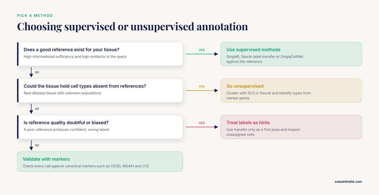
Decision path for cell type annotation: a good reference leads to supervised tools, a doubtful one to unsupervised clustering with marker checks.

A broader comparison investigated eight supervised and ten unsupervised cell type identification methods across fourteen public datasets spanning different tissues, protocols, and species, examining the impacts of cell numbers, cell type count, sequencing depth, batch effects, reference bias, cell population imbalance, and unknown cell types [14]. The central finding is that in most scenarios supervised methods outperform unsupervised methods, except for the identification of unknown cell types [14]. The outperformance holds when the reference dataset has high informational sufficiency, low complexity, and high similarity to the query dataset, and it collapses when the reference is uninformative or biased [14].

The decision rule that follows from these benchmarks:

Use supervised annotation (SingleR, Seurat label transfer, SingleCellNet) when a good reference dataset for your tissue exists.
Use unsupervised approaches when your tissue may contain cell types absent from available references, or when reference quality is doubtful.
Do not treat annotation output as ground truth. Check it against canonical marker genes.

Stage 7: Batch Correction and Dataset Integration

Combining datasets from different batches, donors, or technologies introduces non-biological signals that must be corrected. BatchBench is a modular, flexible R pipeline for comparing batch correction methods, and its authors applied it to eight methods, highlighting methodological differences and assessing performance and computational requirements across well-studied datasets [9]. The framing matters: there is no single best integration method, and the BatchBench pipeline exists so that you can evaluate candidates on your own data rather than trusting generic recommendations.

The practical pros and cons of the two dominant philosophies, expressed qualitatively since the benchmark does not endorse one winner:

Seurat integration anchors datasets together within the Seurat framework and is convenient if you are already in Seurat, at the cost of significant compute on large datasets.
Mutual nearest neighbor and graph-based methods in Bioconductor (for example fastMNN) operate on the SingleCellExperiment object and integrate cleanly into modular pipelines, but require more parameter judgment.

Whatever you choose, run it through a systematic evaluation on your own data before trusting the integrated result, because integration methods can remove genuine biological differences along with batch effects.

Stage 8: Cell-Cell Communication Inference

Cell-cell communication inference predicts ligand-receptor interactions between cell populations from single-cell transcriptomics. This field illustrates how much the choice of package changes the answer.

A systematic comparison of sixteen cell-cell communication resources and seven methods, plus consensus predictions, found few unique interactions among the resources, varying degrees of overlap, and uneven coverage of specific pathways and tissue-enriched proteins [10]. Examining all possible combinations of methods and resources showed that both strongly influence the predicted interactions [10]. The reassuring part is that predictions were generally coherent with spatial colocalization, cytokine activities, and receptor protein abundance [10].

The tool that emerged from this work is LIANA, a ligand-receptor analysis framework providing an open-source interface to all the compared resources and methods [10]. If you are doing communication inference in R, using LIANA is more defensible than committing to a single method, because it lets you check whether your biological conclusion survives a change of method and resource. An earlier version of the same work compared fifteen resources and six methods and reached the same conclusion: the highest ranked interactions differed fundamentally across methods even with the same resources, leading to different biological interpretations [15].

Stage 9: Power Analysis and Study Design

Most analysts discover sample size questions too late. POWSC is an open-source R package for simulation-based power evaluation and sample size recommendation for single-cell RNA-seq differential expression analysis [11]. Its simulator creates realistic expression data capturing the sparsity and heterogeneity of real datasets, and its power assessor provides stratified and marginal power analyses under different comparison scenarios [11]. It also offers information for optimizing the tradeoff between sample size and sequencing depth given a fixed total read budget [11].

The pros: it is the rare design-stage tool purpose-built for scRNA-seq, and it replaces guesswork with simulated power curves. The cons: it covers differential expression specifically, not clustering or annotation power, so it answers one design question thoroughly rather than all design questions.

Platform and Protocol Context

R package choice interacts with the wet-lab platform that produced your data, and several comparisons document this.

Comparisons of technologies from 10x Genomics, PARSE Biosciences, and HIVE for profiling neutrophils in clinical samples found that all methods produced high-quality data capturing neutrophil transcriptomes, and established workflow guidelines for preserving RNA quality in sensitive cell populations [16][17].
A systematic comparison of the 10x Chromium and BD Rhapsody platforms in complex tumors found similar gene sensitivity but differences in mitochondrial content and cell type representation, including a lower proportion of endothelial and myeloid-lineage cells detected by BD Rhapsody and lower gene sensitivity in granulocytes for 10x Chromium [18].
An evaluation of three scRNA-seq approaches for ex vivo drug screening showed variations in library complexity, gene detection sensitivity, and differential expression detection across methods, yet all three consistently recapitulated a transcriptional response to fludarabine in acute lymphoblastic leukemia cells [19].

The takeaway for package selection: before you commit to an annotation or integration package, confirm that the upstream platform bias documented for your chemistry does not interact with the assumptions of that package.

Worked Scenarios

Scenario 1: PBMC immunology dataset with a good human reference

You have 10x data from peripheral blood mononuclear cells and want cell identities. Use Seurat for the backbone, cluster with its graph-based method (a top performer in the twelve-method benchmark [2]), then annotate with SingleR against a curated human reference or Seurat label transfer against a matching dataset. Both are strong performers in the ten-package benchmark [1], and the supervised category wins in this setting because a high-similarity reference exists [14]. Validate top calls with canonical markers such as CD3D, MS4A1, and LYZ.

Scenario 2: Rare disease tissue with unknown cell types

You suspect the tissue contains cell types that no public reference covers. The benchmark evidence says supervised methods lose their advantage exactly here [14]. Run an unsupervised workflow, cluster with SC3 or Seurat [2], and use marker-driven identification rather than forcing reference labels. Use SingleR or Seurat transfer only as a first-pass suggestion, and inspect the unassigned cells manually.

Scenario 3: Multi-donor study with batch effects

You have samples from many donors processed in several batches. Build the pipeline in Bioconductor with SingleCellExperiment so each batch is a normalized object, then run batch correction candidates through a BatchBench-style evaluation on your own data before choosing [9]. Because the best correction method is dataset dependent, and overcorrection can erase real biology, compare candidates empirically rather than by reputation.

Common Mistakes and Limitations

Trusting annotation output without marker validation. Every annotation method benchmarked, including the best performers, makes errors, especially among closely related cell types [1]. Automated labels are hypotheses, not conclusions.

Using a biased or dissimilar reference. Supervised annotation outperformance depends on a reference with high informational sufficiency and high similarity to the query. A poor reference produces confident, wrong labels.

Consensus clustering as a crutch. Averaging multiple clustering methods typically does not improve performance over the best individual method [2]. Effort spent tuning one strong method pays off better.

Ignoring hyperparameter sensitivity in visualization. UMAP and t-SNE results depend on their settings, and nonlinear methods especially require tuning for the specific situation [6]. Two analysts can produce different-looking plots from the same data with no error in either.

Picking a cell-cell communication tool by habit. Predictions change substantially with both the method and the interaction resource used, even on the same dataset [10]. A communication network inferred with one package and one database is a projection, not a map.

Designing the experiment after choosing the software. Power and sample size questions for scRNA-seq differential expression need tools like POWSC at the design stage, and sparsity and heterogeneity make naive bulk-RNA-seq intuition unreliable [11].

Assuming alignment choice is neutral. STAR and Kallisto produce different gene abundance, and the difference propagates into marker detection and annotation [4]. Report which aligner produced your count matrix.

Overlooking framework interactions. Pipeline steps are not independent. The best preprocessing combination in isolation can underperform once steps interact, which is the core motivation for frameworks like pipeComp that evaluate pipelines as wholes [3].

A final limitation applies to all software choices in this field: benchmarks are run on specific datasets with specific properties, and no ranking transfers perfectly to your data. The benchmarks cited here identify which packages deserve first consideration, not which will win on your particular experiment.

Frequently Asked Questions

What is the single best R package for single-cell RNA-seq analysis?

There is no single best package. Seurat is the strongest general framework and performed best at annotating major cell types in a ten-package comparison, but specialist packages such as SC3 for clustering, SingleR for annotation against references, and LIANA for cell-cell communication match or beat it at their specific tasks. Build your backbone with Seurat or Bioconductor and add specialists per stage.

Should I use Seurat or Bioconductor for my first single-cell analysis?

Start with Seurat if you want the fastest path to a complete result, because its end-to-end workflow has the gentlest learning curve and the largest community. Choose Bioconductor if your project needs modular control, multi-package interoperability, or if you plan to compare methods at individual stages. Both are fully production-grade.

Which R package is best for cell type annotation?

SingleR, Seurat label transfer, and SingleCellNet are the strongest evidence-backed choices among single-cell-specific tools, with Seurat best at major cell types and SingleR notably robust to downsampling. The repurposed methylation deconvolution methods CP and RPC also performed well and are legitimate alternatives. Supervised methods win when a good reference exists, and unsupervised approaches are better when unknown cell types may be present.

Do I need to run alignment in R or outside it?

Outside R. STAR and Kallisto, the two most compared alignment approaches, are command-line tools. STAR gives more detected genes and higher expression values but costs roughly 4-fold longer runtime and 7.7-fold more memory than Kallisto. Your aligner choice affects downstream marker detection, so record it and keep it consistent across samples in a study.

How do I choose a batch correction method?

Do not choose by default. BatchBench provides a modular pipeline to compare batch correction methods, and its authors applied it to eight methods across well-studied datasets. The best method depends on your data, so evaluate candidates empirically on your own datasets, checking that biological differences between cell types survive the correction.

How many cells and samples do I need for a single-cell differential expression study?

Use a formal power calculation rather than a rule of thumb. POWSC is an open-source R package that simulates realistic scRNA-seq data and provides power evaluation and sample size recommendations, including the tradeoff between the number of samples and sequencing depth for a fixed total read budget. Sparsity and heterogeneity in single-cell data make intuition carried over from bulk RNA-seq unreliable.