Essential Command-Line Tools for Bioinformatics: A Beginner's Toolkit
By Dr. Zubair Khalid, DVM, MS, PhD ·
The one-sentence difference: a graphical interface asks you to click the same buttons a thousand times, while the command line lets you write down the sequence of steps once and run it on a thousand files. The rule of thumb for choosing where to start: if a task happens once, a web tool is fine, if it happens twice, use the command line, and if it happens three times or involves more than a handful of files, wrap those commands in a script.
This guide covers the basic command line tools bioinformatics beginners actually need, in the order they tend to need them. It is written for someone who has never opened a terminal but who needs to work with sequencing data, whether that is a bacterial genome, an RNA-seq experiment, or a set of variant calls. Every tool described here is free, runs on a standard laptop or an institutional server, and is used daily in real research workflows.
Why Learn Bioinformatics on the Command Line
Most published bioinformatics workflows assume a Linux or Unix environment and describe their steps as typed commands rather than screenshots. A three-day workshop in Cameroon that taught genomics for antimicrobial resistance surveillance included a quick introduction to the Linux command line precisely because web-based tools alone cannot carry a full analysis, and participants showed a substantial increase in confidence after hands-on practice [1]. The same pattern appears across the literature. A beginner-friendly RNA-seq protocol starts with raw FASTQ files and runs its analysis "in command line/terminal and R" [2]. A variant-calling workflow for polyploid plants states plainly that the analysis "begins with preprocessing raw sequencing data" using command-line tools in a Linux environment [3]. A pipeline for African Swine Fever Virus genomes was built so that laboratory professionals "requiring only basic command-line knowledge" could run it [4].
Three practical reasons explain this pattern:
- Reproducibility. A typed command is a record of what you did. You can paste it into a methods section or rerun it next year.
- Scale. A loop that runs one command over 96 sample files takes one line to write and seconds to execute.
- Access to the real tools. FastQC, BWA, GATK, Kraken2, BLAST+, and nearly every program mentioned in sequencing papers are command-line programs. Point-and-click wrappers exist for some of them, but the wrappers lag behind and hide the options you eventually need.
None of this means abandoning graphical tools. Good practice uses both: point-and-click interfaces for exploration and visualization, the shell for anything repetitive or scripted. A study of SARS-CoV-2 Nanopore analysis built its automated trimming, mapping, consensus, and annotation workflow inside the graphical software Geneious Prime specifically because pure command-line pipelines exclude "users with limited programming skills" [5]. That is a legitimate trade-off, and the comparison table later in this article makes it explicit.
Setting Up Your Environment
Terminal, shell, and operating system
The terminal is the window where you type commands. The shell is the program inside it that interprets them, and on virtually every Linux distribution and macOS machine that shell is bash. Linux is the standard for bioinformatics because most server clusters run it and most tools are developed and tested on it first. macOS works nearly identically because it is built on Unix.
On Windows, install the Windows Subsystem for Linux (WSL), which runs a real Ubuntu environment alongside Windows. Do not try to force Windows-native versions of genomics tools, since many assume Unix file paths and utilities.
A basic sanity check once your terminal is open:
pwd        # print working directory, shows where you are
whoami     # your username
uname -a   # operating system and kernel information
Installing software with conda and Bioconda
Manual installation is the fastest way to break a new laptop setup. The practical standard is conda (or the faster Miniforge/mamba variant) together with Bioconda, the community channel that packages thousands of bioinformatics programs. A typical workflow:
conda create -n bio -c conda-forge -c bioconda fastqc seqkit samtools bwa
conda activate bio
fastqc --version
This creates an isolated environment named bio so that incompatible program versions in one project cannot corrupt another. When a paper says it used FastQC and BWA, you can usually install exactly those tools from Bioconda by name.
A text editor and a place to work
Pick one terminal-friendly editor (nano is the gentlest starting point, vim the long-term standard) and learn to open, edit, and save text files. Keep raw sequencing data in a separate read-only directory, keep your analysis scripts under version control with git, and never edit a raw FASTQ file in place.
Core Shell Commands: The Foundation
Every downstream tool assumes you are comfortable with a small set of built-in commands. These are the best basic command line tools bioinformatics beginners can learn first, because every other tool is invoked the same way: a program name, options, then files.
Moving around and looking at files
| Command | What it does | Example |
|---|---|---|
pwd | Print the current directory | pwd |
ls | List files. -l adds details, -lh shows human-readable sizes | ls -lh data/ |
cd | Change directory. cd .. goes up one level | cd results/ |
mkdir | Create a directory | mkdir -p results/qc |
cp, mv, rm | Copy, move or rename, delete. rm does not ask twice and has no undo | mv sample1.fastq.gz raw/ |
head, tail | Show the first or last lines. -n 20 sets the count | head -n 8 sample.fastq |
less | Scroll through a file interactively. Press q to quit | less assembly.fasta |
wc | Count lines, words, or characters. -l counts lines | wc -l counts.txt |
du, df | Disk usage of files, and free space on disks | du -sh raw/ |
Two habits matter more than memorization. First, use tab completion: typing sam and pressing Tab completes to samtools and shows matching files. Second, treat rm with respect. A sequencing run can cost thousands of dollars, and rm -rf applied to the wrong directory has destroyed more data than any disk failure.
FASTQ structure and why line counting matters
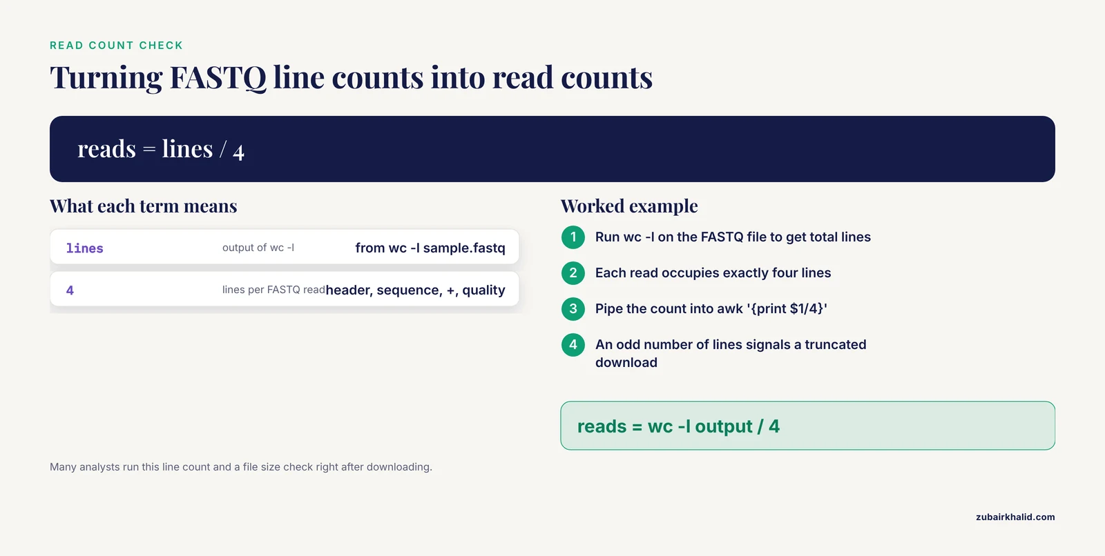
A FASTQ file stores sequencing reads with a quality score for every base. Each read occupies exactly four lines:
@READ_ID_1
GATCGATCGATC...
+
IIIIIIIIIIII...
This is why wc -l sample.fastq | awk '{print $1/4}' gives you the read count, and why an odd number of lines in a FASTQ almost always means a truncated download. After downloading data, the first command many analysts run is a line count and a file size check.
Pipes and redirection: combining small tools
The shell's real power comes from two operators. The pipe | sends the output of one command into the input of the next. Redirection with > writes output to a file, and >> appends to one.
# Count sequences in a FASTA file (headers start with >)
grep -c ">" assembly.fasta

# Extract the 10 most common lengths of reads in a FASTQ
awk 'NR%4==2{print length($0)}' reads.fastq | sort | uniq -c | sort -rn | head

# Save a filtered list for later
grep "control" samples.tsv > control_samples.txt
Each piece is trivial. Chained together they replace what would otherwise be a custom script.
Text Processing Tools: grep, sed, awk, cut, sort, uniq
Sequencing data is text, so text tools are sequencing tools. These are the options that make command-line fluency possible, and they appear in essentially every published workflow that touches raw files.
grep: find lines that match
grep prints lines matching a pattern. In bioinformatics it finds reads with a barcode, pulls specific chromosome entries out of a GFF annotation, or counts headers in a FASTA.
grep -c ">" genome.fasta          # number of sequences
grep "chr1" annotations.gff       # all chr1 features
grep -v "N" reads.fastq           # lines without an N (careful: this includes headers)
Useful options: -v inverts the match, -c counts instead of printing, -A 1 prints one line after each match (handy for grabbing the sequence line under a header), and -f patternfile.txt matches any pattern listed in a file.
cut, sort, uniq: columns and summaries
Tab-separated tables (sample sheets, count matrices, BLAST output) respond well to this trio.
# Second column of a tab-separated sample sheet
cut -f2 samples.tsv

# Unique values in column 3, counted
cut -f3 annotations.gff | sort | uniq -c
sort must run before uniq counts unique values, which is the single most common ordering mistake beginners make.
awk: the workhorse for columnwise operations
awk processes files line by line, splits each line into fields ($1, $2, and so on), and can filter, compute, and format in one pass. For many beginners, learning ten lines of awk pays off more than a month of any other tool.
# Total length of all sequences in a FASTA (assumes one line per sequence)
awk '/^>/{next}{total += length($0)} END{print total}' genome.fasta

# GC content of a single-sequence FASTA
awk '!/^>/{gc += gsub(/[GC]/,""); n += length($0)} END{print gc/n}' genome.fasta

# Print rows of a table where column 5 exceeds 0.05
awk '$5 > 0.05' differential_results.tsv
sed: targeted editing
sed performs substitutions across a file. The classic use is cleaning identifiers:
# Replace underscores with hyphens in sample names throughout a VCF header
sed 's/_/-/g' sample_names.txt

# Strip the first character from every line of a file
sed 's/^.//' file.txt
Run sed on a copy until you trust the pattern. sed -i edits files in place and cannot be undone.
When to graduate to a scripting language
Once a one-liner grows past two or three operations, write it as a script. Bash scripts are the natural next step, and published pipelines are routinely "executed locally through bash scripts, or using a Slurm protocol for batch processing" [4]. Python and R follow. The command line does not compete with Python and R, it is the environment where their tools live, and a workflow designed "for researchers with basic familiarity with command-line tools and R programming" reflects how real analysis actually splits [6].
Knowing Your File Formats
Half of beginner confusion is format confusion. Learn to recognize these five by sight and the rest of bioinformatics becomes mostly lookups.
| Format | Stores | Structure | Common tools that read it |
|---|---|---|---|
| FASTA | Reference genomes, assembled contigs, protein sequences | Header line starting with >, then sequence lines | grep, SeqKit, BLAST+, BWA |
| FASTQ | Raw reads plus per-base quality scores | 4 lines per read: header, sequence, +, quality | FastQC, trimmers, aligners |
| SAM / BAM | Aligned reads against a reference | SAM is text, BAM is its compressed binary form | samtools, IGV (visual) |
| VCF / BCF | Variant calls with per-sample genotypes | Header block starting ##, then one variant per line | bcftools, vembrane, SnpEff |
| GFF/GTF | Gene and feature annotations | Tab-separated, 9 columns per feature | awk, grep, genome browsers |
BAM and BCF are the binary forms of SAM and VCF. They are smaller and faster to query, and the bcftools view and samtools view commands convert between text and binary forms on demand. When a file has an index partner (.bam.bai, .bcf.csi), the index lets tools jump directly to a genomic region instead of reading the whole file.
The Core Bioinformatics Command-Line Programs
This section covers the programs a working analyst touches in nearly every project. Each subsection states what the tool does, the most useful basic options, and its strengths and weaknesses.
FastQC: quality control as a first reflex
FastQC summarizes per-base quality scores, adapter contamination, sequence duplication, GC content, and overrepresented sequences in a raw FASTQ file [3]. You run it on every sample before anything else.
fastqc *.fastq.gz -o qc_reports/Pros: fast, universally cited, HTML reports a reviewer can read. Cons: it reports characteristics, not decisions. A high per-base quality drop at read ends is normal for many chemistries, so FastQC flags require interpretation in context, usually confirmed with a summarizer like MultiQC across all samples.
Read trimming: Trim Galore and friends
Trimming removes adapters and low-quality bases before alignment. Trim Galore wraps the FastQC metrics and the Cutadapt trimmer and is the tool named in a published Illumina variant-calling workflow for "optional adapter and low-quality sequence removal" [3].
trim_galore --paired sample_R1.fastq.gz sample_R2.fastq.gzPros: one command handles paired-end logic and adapter detection. Cons: over-trimming discards real data, and some modern aligners tolerate low-quality tails well enough that aggressive trimming can hurt more than help. Trim for adapters, trim conservatively for quality.
Aligners: BWA and minimap2
An aligner maps each read to a reference genome. For Illumina short reads, the published plant-genomics workflow uses BWA for sequence alignment [3]:
bwa index reference.fa
bwa mem reference.fa sample_R1.fastq.gz sample_R2.fastq.gz > sample.sam
For Nanopore and PacBio long reads, minimap2 is the standard. Aligners convert SAM output through samtools into sorted, indexed BAM files:
samtools sort sample.sam -o sample.sorted.bam
samtools index sample.sorted.bam
samtools flagstat sample.sorted.bam   # mapping statistics summary
Pros: these are the reference-standard tools behind thousands of papers, thoroughly validated, and fast enough for whole genomes on a laptop (bacterial) or a server (human). Cons: aligner choice depends on read type and genome, and a mis-specified reference genome produces confident-looking garbage alignments. Always check flagstat output before trusting downstream calls.
samtools and bcftools: the BAM and VCF toolbox
samtools manipulates alignments (sorting, indexing, extracting regions, pileups) and bcftools manipulates variant calls (viewing, filtering, merging, consensus generation). Together they are the most-used utilities in genomics.
samtools view -c sample.sorted.bam chr1          # reads on chr1
bcftools view -i 'QUAL>30' variants.bcf          # variants above Q30
A companion tool in the same spirit is vembrane, which filters VCF/BCF files with Python expressions and "exposes the VCF/BCF file type specification" as Python data structures, requiring only basic Python knowledge, and runs fast through lazy evaluation [7]. If your filtering logic involves annotation fields from SnpEff or VEP, vembrane expresses it cleanly.
Variant calling and annotation: GATK and SnpEff
The published polyploid plant workflow performs "variant calling using the Genome Analysis Toolkit (GATK)", then filters false positives and annotates "with SnpEff" [3]. GATK implements statistical models for calling variants from aligned reads, including joint calling across sample batches. SnpEff predicts which genes a variant affects.
gatk HaplotypeCaller -R reference.fa -I sample.sorted.bam -O sample.vcf
snpEff coffea_arabica sample.vcf > sample_annotated.vcf
Pros: GATK's best-practice documentation is exceptional, and annotation turns a pile of positions into biological hypotheses. Cons: GATK workflows involve many steps with strict input requirements, and polyploid genomes require parameter choices that differ from diploid defaults.
BLAST and BLAST-like searchers
BLAST finds sequence similarity. BLAST+ is the standard command-line suite:
makeblastdb -in ref_proteins.fa -dbtype prot
blastp -query my_protein.fa -db ref_proteins -outfmt 6 -evalue 1e-5
The -outfmt 6 tabular output feeds directly into cut and sort. A portable alternative is nsearch, a BLAST-like algorithm available as a command-line tool, a Python package (npysearch), and an R package (Blaster), benchmarked as comparable in speed and accuracy to BLAST+ and VSEARCH [8]. Its value is embedding: if you build a web app or pipeline that needs similarity searches, nsearch libraries slot into Python and R frameworks directly.
Pros of BLAST-family tools: universal, flexible across nucleotide and protein searches, and the de facto language of homology. Cons: e-values are easily misread as probabilities, and BLAST output columns vary by format code, so always confirm column order before parsing.
SeqKit: FASTA/FASTQ statistics in one line
SeqKit reports sequence counts, length distributions, GC content, and more, and can filter sequences by length. The SeqLengthPlot authors describe SeqKit as "a very complete and fast tool for sequence analysis" while noting limits such as returning sequences only shorter or only longer, not both at once, for a given cutoff [9]. That gap is exactly why SeqLengthPlot v2.0 was written as an all-in-one Python tool that splits FASTA files by a length cutoff, plots the length distribution, and prints statistics [9].
seqkit stats assembly.fasta
seqkit seq -n assembly.fasta | head    # sequence names
Pros: fast, single static binary, no dependencies. Cons: it is a statistics and manipulation layer, not an analysis engine.
Taxonomic classification: Kraken2 and Krona
Kraken2 classifies sequencing reads against a database of reference genomes using exact k-mer matches, and Krona turns classification output into interactive, collapsible pie visualizations. A published Nanopore protocol for plant pathogen genomics describes "command-line analyses with Kraken2 and Krona" within a modular pipeline for genome assembly, annotation, and taxonomic identification, alongside the more graphical EPI2ME tools [10].
kraken2 --db minikraken_db reads.fastq.gz --output kraken.tsv --report kraken.report
ktUpdateTaxonomy.sh   # keep taxonomy files current before building reports
Pros: extremely fast, works on raw reads, and Krona output is genuinely intuitive. Cons: results are only as good as the database, exact-match classifiers struggle with novel organisms, and database builds consume significant disk space.
Alignment-free phylogenetics: TreeWave
Not every comparison needs an alignment. TreeWave reconstructs phylogenies from frequency chaos game representations and discrete wavelet transforms of sequences, an alignment-free approach validated on virus, bacterial, human mitochondrial, and rRNA datasets, with a significant reduction in running time on large datasets and classification accuracy similar to classical multiple-sequence-alignment methods [11].
Pros: open source, user-friendly CLI, faster and more scalable than MSA-based pipelines for large sets of genomes. Cons: alignment-free summaries can miss alignment-specific biology, and MSA-based trees remain the expectation in many journals.
Metagenomics pipelines: bioBakery and friends
For shotgun metagenomics, an unbiased comparison of mock-community performance tested bioBakery, JAMS, WGSA2, and Woltka. bioBakery4 performed best on most accuracy metrics, and the authors noted that bioBakery "is commonly used and only requires a basic knowledge of command line usage" [12]. That last sentence is a useful signal: a tool with modest command-line demands that tops accuracy benchmarks is an ideal beginner target.
Data retrieval: getSequenceInfo
Before analysis you need data. getSequenceInfo (gSeqI) retrieves sequence information and data from GenBank, RefSeq, and the European Nucleotide Archive, runs on Linux, macOS, and Windows, works programmatically from the command line or through a GUI, separates chromosomes from plasmids into folders, and computes basic statistics such as GC content [13]. Pros: multi-repository, cross-platform, dual interface. Cons: it retrieves and organizes, it does not analyze.
Side-by-Side Comparison: How Your Options Actually Differ
The choice that structures every beginner's path is not which single tool to learn but which interface and workflow style to invest in. The table below compares the four main ways of getting bioinformatics work done.
| Criterion | Command line (shell tools) | Command-line bioinformatics programs | Web servers and GUIs | Workflow managers and pipelines |
|---|---|---|---|---|
| Representative examples | grep, awk, sed, sort, pipes | FastQC, BWA, samtools, bcftools, BLAST+, SeqKit, Kraken2 [15] | Galaxy-style servers, Geneious Prime workflows, CRISPR-GRANT, rna-tools.online [4][5][9] | Snakemake, Nextflow, bash-plus-Slurm pipelines like PePApipe [4] |
| Best suited to | File manipulation, QC one-liners, data hygiene | The actual analysis steps (QC, alignment, calling, classification) | One-off analyses, novices, teaching demonstrations | Multi-sample, multi-step, repeated projects |
| Reproducibility | High if commands are saved in scripts | High, all parameters visible | Low to moderate, clicking is rarely recorded | Highest, the pipeline file is the methods section |
| Learning curve | Days to weeks | Weeks per tool family | Hours | Weeks, but builds directly on CLI tools |
| Scale (96 samples) | Manual loops, workable | Excellent, built for it | Often impractical or costly | Excellent, often with parallelism |
| Transparency | Total, you see every step | Total | Partial, defaults are hidden | Total, if you read the pipeline |
| Main risk | Destructive typos (rm, in-place edits) | Silent wrong-parameter results | Unrecorded choices, version drift | Black-box use without understanding the steps |
| Where beginners should start | First | Second | Fine for exploration, not as the final skill | Last, after the component tools make sense |
Published tools exist at every point on this spectrum by design. CRISPR-GRANT was created because existing indel analysis tools required "certain bioinformatics training and basic command-line processing capability," and its GUI "significantly lowers the barrier" for wet-lab researchers [14]. rna-tools.online moved RNA 3D modeling tasks to a web server because the underlying rna-tools package "requires the installation of a mixture of libraries and tools, basic knowledge of the command line and the Python programming language" [15]. Both are good tools. Both also demonstrate the pattern: graphical options trade flexibility for accessibility, and analysts who eventually need the flexibility return to the command line.
Worked Scenarios
Scenario 1: Your first RNA-seq analysis
You have six FASTQ files from a mammalian cell experiment. The published beginner protocol walks exactly this path, starting "from raw .fastq files" with quality control, trimming, alignment to the genome, and gene quantification, followed by differential expression and visualization in R via RStudio, with all code explained step by step [2]. In concrete terms: run FastQC on all six files, view the reports, trim adapters, align with a splice-aware aligner, quantify genes, then move the count matrix into R. Your command-line contribution is the first half, your R contribution the second, and the protocol demonstrates that this split is standard rather than exceptional [2].
The realistic time investment for a first pass is a few days, most of it spent understanding why each step exists rather than typing the commands.
Scenario 2: Variant calling in a non-model genome
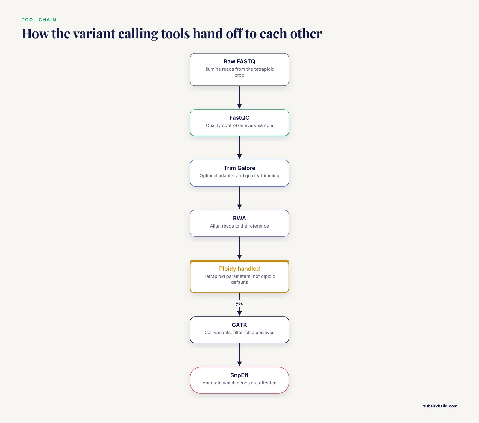
You sequence a tetraploid crop species with Illumina reads and want mutation-induced SNVs. The published workflow runs entirely on the Linux command line, preprocessing raw data with FastQC and optional Trim Galore, aligning with BWA, calling variants with GATK, filtering false positives, and annotating with SnpEff, with the polyploid nature of the genome handled explicitly at the calling step [3]. This scenario illustrates two lessons. First, the tool chain (FastQC to Trim Galore to BWA to GATK to SnpEff) is a chain, each tool consuming the previous tool's output. Second, biological context, here ploidy, changes parameters, which means you must understand the tools rather than copy a human-genome tutorial blindly.
Scenario 3: Public health genomics without a cluster
A surveillance laboratory receives bacterial isolates for antimicrobial resistance analysis. The Cameroon workshop approach combined web-based tools for AMR prediction and phylogenetics with a foundation of NGS concepts, file formats, data sharing, and a Linux command line introduction [1]. The realistic takeaway for a small lab is that web tools can carry more of the load than purists admit, but the command-line foundation is what lets staff move data between tools, reformat files, and sanity-check outputs. Capacity-building programs target that foundation deliberately.
Scenario 4: Scaling up to an automated pipeline
You now analyze ASFV genomes routinely and want consistency. PePApipe integrates thirteen software tools into one automated Python-driven workflow covering quality control, preprocessing, de novo assembly, and variant calling, executed locally through bash scripts or via Slurm for batch processing, and it classifies outputs into structured folders while retaining intermediate files for further analysis [4]. The design lesson is that a good pipeline is not magic, it is your manual commands written down, ordered, and made sample-aware. You cannot debug a pipeline you could not have run by hand.
Scenario 5: Rapid pathogen detection in the field
You sequence a blueberry pathogen on a MinION and need to know what it is within hours. The published protocol describes a modular pipeline spanning the user-friendly EPI2ME tools to command-line analyses with Kraken2 and Krona for taxonomic identification, plus genome assembly and comparative work [10]. Modularity is the point: you can run the graphical layer for the urgent diagnostic call and the command-line layer for the publishable characterization, without converting your data.
Beyond Single Commands: Scripts, Job Schedulers, and Workflows
Once individual commands feel comfortable, three layers of structure await, in this order.
Bash scripting. Put your commands in a .sh file, add a for loop over sample names, and you have a pipeline for one sample type. Add variables, if checks, and argument parsing gradually. Every serious pipeline started as a bash script, and ASFV analysis pipelines are still distributed this way for local execution [4].
Job schedulers. When your institution provides a compute cluster, Slurm submits your script as a job with a resource request. The PePApipe protocol ships a Slurm variant for batch processing of multiple samples [4]. Learn sbatch, squeue, and scancel, and never run a whole-genome alignment on a shared login node.
Workflow managers. Snakemake (Python-based) and Nextflow (compatible with containers and cloud execution) turn pipelines into files that track dependencies, skip completed steps, and document software versions. Adopt one once you find yourself rerunning 15 steps because step 3 changed. The mock-community metagenomics evaluation that compared bioBakery4, JAMS, WGSA2, and Woltka exemplifies the modern reality that pipelines, not single tools, are what get benchmarked [12].
A note on learning resources: a structured bioinformatics course, whether a university module, a Software Carpentry workshop, or a protocol-style walkthrough with provided code [2], compresses months of self-teaching into weeks. Protocol journals such as Current Protocols publish step-by-step, command-level guides for variant calling [3], pathogen genomics [10], and transcriptomics [2], and those are close readings of the actual keystrokes rather than abstract overviews.
Common Mistakes and Limitations
These are the errors that consume the most beginner time, listed so you can avoid each specifically.
- Editing or deleting raw data. Never write to the directory holding raw FASTQ/BAM files. Copy, analyze, and keep originals read-only.
- Trusting output you have not inspected.
headevery output file. A tool that exits without an error message has still, sometimes, produced an empty or truncated file because an earlier step quietly failed. - Spaces in filenames. A file named
sample 1.fastq.gzbreaks loops and quoted arguments in ways that are miserable to debug. Use underscores from the start. - Parsing with assumptions about columns. Always confirm column order in BLAST
-outfmt 6tables, GFF files, and VCF annotation fields before writing awk or cut commands against them. - Confusing e-values, p-values, and identity percentages in similarity searches, or reading a low e-value as proof of functional equivalence.
- Over-trimming reads, then blaming the aligner for poor mapping. Check mapping statistics with
flagstatbefore and after trimming. - Treating FastQC warnings as failures. FastQC reports characteristics, and module flags depend on read length and library type. Interpret, do not panic.
- Not recording software versions.
conda env export > environment.ymlafter installing. A methods section without versions is not reproducible. - Copying tutorials without adapting to your organism. Parameters for a human diploid genome do not transfer to a tetraploid plant [3], a bacterial genome, or a mixed metagenome.
- One limitation applies to this entire toolkit: the command line accelerates analysis but does not decide it. Tool choices, parameter thresholds, and biological interpretation remain the analyst's responsibility, and study designs with specific questions need domain expertise and, where relevant, professional involvement appropriate to the field.
Frequently Asked Questions
Do I need to know programming before I learn bioinformatics?
No. The command line is the entry point, and it is a skill of vocabulary and pattern recognition rather than programming logic. Many published beginner workflows explicitly assume only "basic command-line knowledge" or basic familiarity alongside R [6][7][8]. Start with the shell commands above, add R or Python after your first real analysis.
What are the best basic command line tools bioinformatics beginners should learn first?
In order: the navigation and file commands (ls, cd, head, less, wc), then grep, cut, sort, uniq, and basic awk, then FastQC, SeqKit, and samtools as your first domain tools. This ordering mirrors how beginner protocols actually teach the work, quality control first, then processing [15].
Command line versus graphical tools, what are the pros and cons?
Command line offers reproducibility, scale, and direct access to the tools papers use, at the cost of a steeper learning curve and destructive-typos risk. Graphical tools like Geneious Prime workflows and CRISPR-GRANT lower the barrier dramatically and suit one-off analyses, but record fewer choices and scale poorly [4][9]. The practical resolution is to use both, with the shell as the backbone.
Which operating system should I use?
Linux, or macOS, or Windows with WSL running Ubuntu. Nearly all sequencing tools are developed for Unix-like systems, and server clusters run Linux, so comfort in a bash shell transfers directly to every high-performance environment you will later encounter.
How long does it take to become productive on the command line?
A focused beginner can navigate files, run FastQC, and chain simple text tools within two to three weeks of regular practice. Running a complete, correct variant-calling or RNA-seq workflow typically takes a few months, which is why protocol-style guides with provided code accelerate the process so effectively [15].
Is a formal bioinformatics course necessary, or can I self-teach?
Self-teaching works, and free workshops and protocol guides exist for exactly this purpose, with documented confidence gains from structured hands-on workshops [1]. A formal course or workshop adds structure, feedback, and a community, which matters most for debugging. If you self-teach, follow a written, command-level protocol end to end before improvising [2].
Sources
- Enable, empower, succeed: a bioinformatics workshop Harnessing open web-based tools for surveillance of bacterial antimicrobial resistance.
- A Guide to Basic RNA Sequencing Data Processing and Transcriptomic Analysis.
- Single Nucleotide Variant Calling in Polyploid Plant Genomes From Illumina Short Reads: A Practical Workflow Illustrated With Coffea arabica L.
- 'PePApipe': A complete bioinformatics analysis pipeline for African Swine Fever Virus genome.
- From SARS-CoV-2 to Global Preparedness: A Graphical Interface for Standardised High-Throughput Bioinformatics Analysis in Pandemic Scenarios and Surveillance of Drug Resistance.
- Bioinformatics Workflow for Co-Transcriptome Analysis of Plant-Bacterial Interactions.
- Insane in the vembrane: filtering and transforming VCF/BCF files.
- Portable BLAST-like algorithm library and its implementations for command line, Python, and R.
- SeqLengthPlot v2.0: an all-in-one, easy-to-use tool for visualizing and retrieving sequence lengths from FASTA files.
- MinION Nanopore-Enabled Identification and Genomic Characterization of Pseudomonas syringae Complex Infecting Blueberry Using Symptomatic Plant Samples and Pathogen Pure Culture.
- TreeWave: command line tool for alignment-free phylogeny reconstruction based on graphical representation of DNA sequences and genomic signal processing.
- Mock community taxonomic classification performance of publicly available shotgun metagenomics pipelines.
- getSequenceInfo: a suite of tools allowing to get genome sequence information from public repositories.
- CRISPR-GRANT: a cross-platform graphical analysis tool for high-throughput CRISPR-based genome editing evaluation.
- rna-tools.online: a Swiss army knife for RNA 3D structure modeling workflow.