Analyzing Protein-Protein Interfaces in AlphaFold Structures
By Dr. Zubair Khalid, DVM, MS, PhD ·
By the end of this tutorial you will be able to take an AlphaFold-predicted complex, locate exactly which residues form the interface between two chains, quantify that interface with buried surface area and contact counts, judge whether the interface is actually well supported by the model's own confidence metrics, and rank competing models of the same interaction. You will also learn how researchers map disease mutations onto predicted interfaces and how to spot the failure modes that produce convincing-looking but wrong interfaces.
This guide assumes you have a machine with Python 3.9 or newer, the ColabFold package or access to the AlphaFold 3 web service, and the Biopython and SciPy libraries. Everything else runs on a laptop.
What You Need Before You Start
Install the analysis dependencies with pip or conda:
pip install biopython scipy numpyFor running predictions yourself, ColabFold wraps AlphaFold-Multimer in a scriptable command-line tool:
conda install -c conda-forge colabfoldA protein-protein interaction (PPI) is a durable or transient physical association between two or more protein chains. An interface is the set of residues, one or more from each chain, whose atoms come into close contact when the proteins bind. AlphaFold-Multimer (often abbreviated AFM) is the multi-chain extension of AlphaFold 2 that predicts the structure of such assemblies, and it has become a standard tool both for modeling known complexes and for discovering previously unknown PPIs at scale [1].
Three routes lead to a structure you can analyze:
- The AlphaFold Protein Structure Database, which holds predicted single-chain structures for complete proteomes and can be downloaded without running any prediction.
- The AlphaFold 3 server, a web service where you paste sequences and receive predicted complexes, useful for small numbers of pairs when you have no local compute [2], [3].
- Local pipelines such as ColabFold or AlphaPulldown, which you need for anything beyond a handful of pairs.
This walkthrough uses ColabFold outputs because their PAE and ipTM values are stored in a convenient JSON format, but the interface-extraction and scoring steps work identically on AlphaFold 3 server downloads and on AlphaPulldown results.
How AlphaFold Reports Confidence at Interfaces
Before touching any coordinates, you need to understand the three numbers that ship with every AlphaFold-Multimer prediction, because they decide how much you should trust the interface you are about to analyze.
Predicted TM-score (pTM) estimates, on a 0 to 1 scale, how accurately the overall topology of the full assembly is predicted. Interface pTM (ipTM) applies the same logic specifically to residues that span chain boundaries, so an ipTM near 1 means the model is confident about the relative placement of the interacting chains. Predicted Aligned Error (PAE) is a matrix with one value for every pair of residues, given in Angstrom units, estimating the expected positional error at one residue if the model were aligned on the other. Low PAE between residues on different chains is the clearest signal that a specific interface, not just a generic association, was predicted confidently.
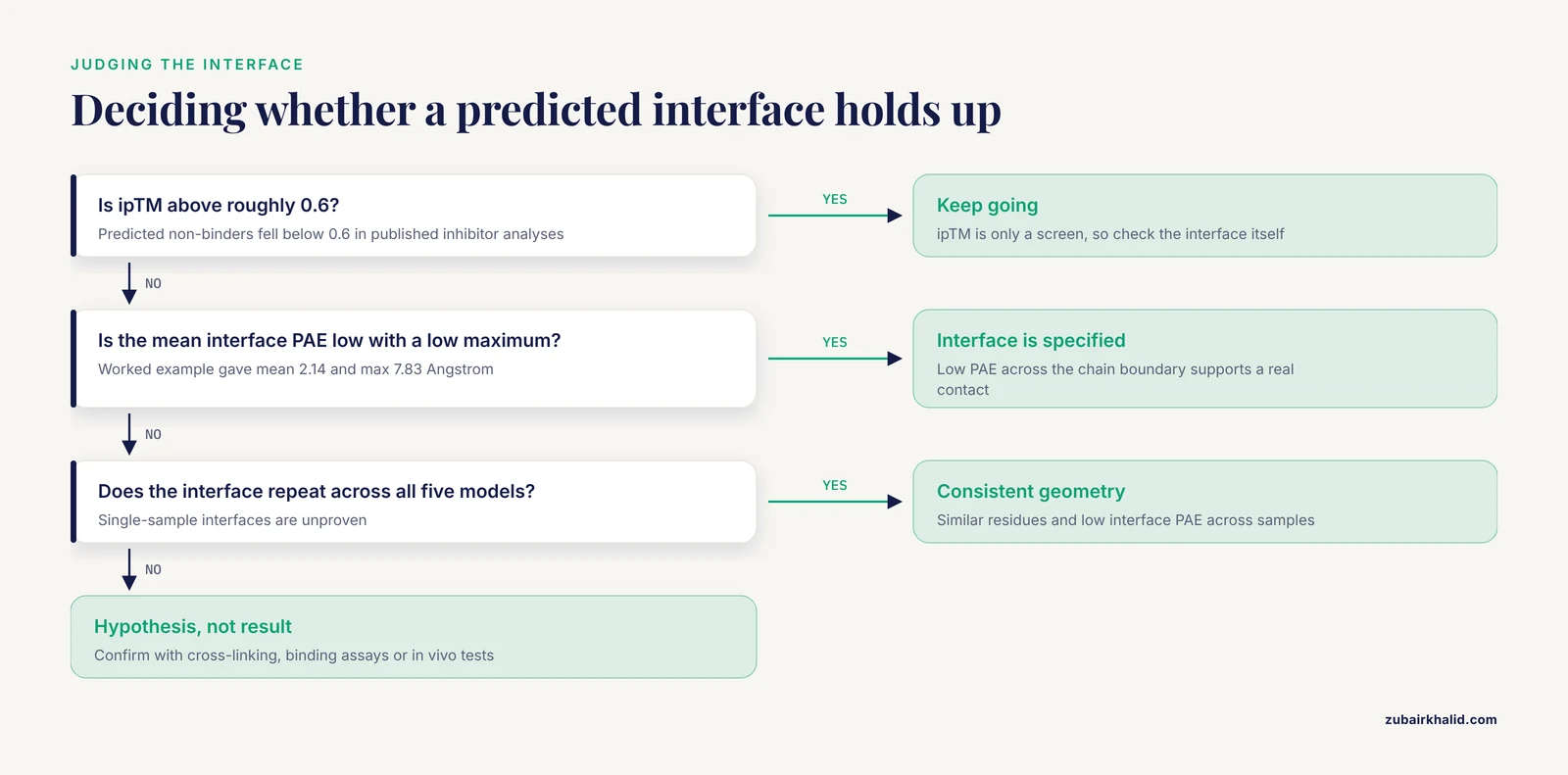
The distinction matters because ipTM has a documented blind spot. A re-evaluation of high-confidence Drosophila and human PPI datasets found that ipTM reflects overall structural integrity but can miss physiologically relevant interactions that involve small interfaces or flexible regions. The authors therefore introduced the Local Interaction Score (LIS), which is derived from the PAE matrix and focuses on regions with low PAE values, and showed that this improves detection of interactions at small and flexible interfaces [4]. A later analysis of plant Kunitz inhibitor-trypsin pairs illustrates the usual behavior of ipTM where it does work well: predicted binders scored between 0.77 and 0.82, while predicted non-binders fell below 0.6 [5]. Treat ipTM as a coarse filter and PAE-based local measures as the fine instrument.
| Metric | What it tells you | Where it comes from | Typical use |
|---|---|---|---|
| , - | , - | , - | , - |
| pTM | Confidence in overall assembly topology | Model output JSON | Coarse sanity check of the whole complex |
| ipTM | Confidence in cross-chain residue placement | Model output JSON | First-pass filter for whether the pair binds |
| PAE | Expected positional error for every residue pair, in Angstroms | Model output JSON or PNG | Identifies which interface is real inside a model |
| Mean interface PAE | Average PAE restricted to cross-chain interface residue pairs | Computed from PAE matrix and your residue list | Local confidence at the specific interface you care about |
| Buried surface area | Solvent-accessible area hidden from water upon binding | Computed from coordinates with Shrake-Rupley SASA | Physical plausibility and interface size |
| Contact count | Number of residues touching across chains | Computed from coordinates with a distance cutoff | Quick interface size and residue listing |
Where to Get Structures for Protein-Protein Interaction Analysis
For a single known or suspected pair, the fastest path is the AlphaFold 3 server. You paste the sequences of the chains, the service runs the model, and you download the resulting structure and its confidence data. Benchmarks of cofolding methods that were not specifically trained on ternary complexes found AlphaFold 3 achieving the best overall performance for PPI interface prediction among the tested models, ahead of Boltz-1, Chai-1, Protenix, and RoseTTAFold All-Atom [3], which makes it a reasonable default for small jobs. The server does enforce usage constraints, so it does not scale to screening campaigns.
For larger projects, two packages dominate. AlphaPulldown is a Python package built around AlphaFold-Multimer that streamlines PPI screens and high-throughput modeling of higher-order oligomers, provides a command-line interface, a variety of confidence scores, and a graphical analysis tool [1]. If you prefer a browser over a terminal, AlphaPPIweb wraps AlphaPulldown in a web platform where users input amino acid sequences and receive three-dimensional predictions, confidence scores, automated interface residue analysis, and bait-versus-candidate screening for ligand-receptor style questions [6].
A third consideration is stoichiometry. A binary model answers only whether chain A can touch chain B. Whether that contact survives inside a larger assembly, and whether a partner competes for the same surface, depends on modeling context. MultimerMapper addresses exactly this by generating ensembles of overlapping structure predictions, then using graph-based analysis to infer stoichiometries, highlight higher-order subassemblies, and identify alternative interaction modes and conformational changes associated with the presence or absence of specific partners [7]. If your biological question involves a protein with many possible partners, budget time for this kind of ensemble analysis rather than a single pairwise run.
AlphaFold Protein-Protein Interaction Interface Analysis Step by Step
The worked example below analyzes a two-chain prediction. Substitute your own sequences and file names throughout.
Step 1. Prepare the FASTA and Run the Prediction
AlphaFold-Multimer takes a multi-chain FASTA file. Save your two chains as complex.fasta:
>sp|P12345|chain_A protein A
MKTAYIAKQRQISFVKSHFSRQ
>sp|Q9XXXX|chain_B protein B
MKWESPFKVAPAEFQ
Run ColabFold with the multimer model:
colabfold_batch complex.fasta af2_out \
  --model-type alphafold2_multimer_v3 \
  --num-models 5 \
  --num-recycle 3
The two parameters that matter most are:
-model-type alphafold2_multimer_v3selects the multimer weights. Running the monomer model on a two-chain FASTA either fails or produces meaningless per-chain outputs.-num-models 5generates five independent structure samples. Multimer predictions are stochastic, and different seeds can place the same chains in different orientations, so a single model is never sufficient for interface conclusions.
After the run finishes, the output directory contains, depending on your ColabFold version, files named like this:
af2_out/
  ranked_0.pdb
  ranked_0_scores.json
  ranked_0.pae.png
  ranked_1.pdb
  ranked_1_scores.json
  ...
The ranked_*.pdb files are the five models ordered by the tool's internal ranking, and each *_scores.json carries the pTM, ipTM, and full PAE matrix for that model.
Step 2. Read the Confidence Outputs
Load the best-ranked model's score file:
import json

with open("af2_out/ranked_0_scores.json") as handle:
    scores = json.load(handle)

print("ipTM:", round(scores["iptm"], 3))
print("pTM:", round(scores["ptm"], 3))
Expected output for a well-predicted dimer looks like this:
ipTM: 0.81
pTM: 0.74
How to interpret it: an ipTM above roughly 0.6 is commonly used in the literature as a first-pass sign of a predicted interaction, and predicted non-binders in published inhibitor analyses fell below that level, while confident binders scored in the high 0.7s [5]. Use it only as a screen. As the next steps show, the PAE matrix contains far more decision-relevant information than the single ipTM number.
Step 3. Locate the Interface Residues
The most direct definition of an interface is geometric: residues whose heavy atoms lie within a short distance of atoms on the other chain. A heavy-atom cutoff of 4.5 Angstroms is a common convention for protein-protein contacts. The following script reads a PDB file, builds a spatial index with SciPy, and reports the interface residues for each cross-chain pair. It also writes per-chain residue lists that later steps reuse.
from collections import defaultdict

import numpy as np
from Bio.PDB import PDBParser
from scipy.spatial import cKDTree

CUTOFF = 4.5  # Angstroms, heavy-atom contact convention

parser = PDBParser(QUIET=True)
structure = parser.get_structure("complex", "af2_out/ranked_0.pdb")

chains = defaultdict(list)
for atom in structure.get_atoms():
    if atom.element == "H":
        continue
    residue = atom.get_parent()
    if residue.id != " ":  # skip waters and hetero residues
        continue
    chain_id = residue.get_parent().id
    chains[chain_id].append((residue.id[4], residue.resname, atom))

ids, coords, chain_of = [], [], []
for chain_id in sorted(chains):
    for resnum, resname, atom in chains[chain_id]:
        ids.append((chain_id, resnum, resname))
        coords.append(atom.coord.tolist())
        chain_of.append(chain_id)

coords = np.array(coords)
tree = cKDTree(coords)
cross_pairs = tree.query_pairs(CUTOFF)

contacts = defaultdict(set)
for i, j in cross_pairs:
    if chain_of[i] == chain_of[j]:
        continue
    contacts[(chain_of[i], chain_of[j])].add(ids[i][4])
    contacts[(chain_of[j], chain_of[i])].add(ids[j][4])

for (c1, c2), residues in sorted(contacts.items()):
    print(f"interface {c1}-{c2}: {len(residues)} residues in chain {c1}")
    with open(f"interface_{c1}_vs_{c2}.txt", "w") as out:
        for resnum in sorted(residues):
            label = next(i for i in ids if i == c1 and i[4] == resnum)
            out.write(f"{resnum}\t{label[1]}\n")
Expected output for a compact heterodimer:
interface A-B: 38 residues in chain A
interface B-A: 31 residues in chain B
Two practical points. First, AlphaFold output has one model per file, so the loop over structure.get_atoms() needs no model handling. Second, remember that residue numbering in the PDB reflects the exact sequence you submitted. If you trimmed a signal peptide or a His-tag before prediction, the numbers in the file start at your first submitted residue, not at UniProt numbering. Map your numbering explicitly before comparing against annotations.
Step 4. Quantify the Interface With Buried Surface Area
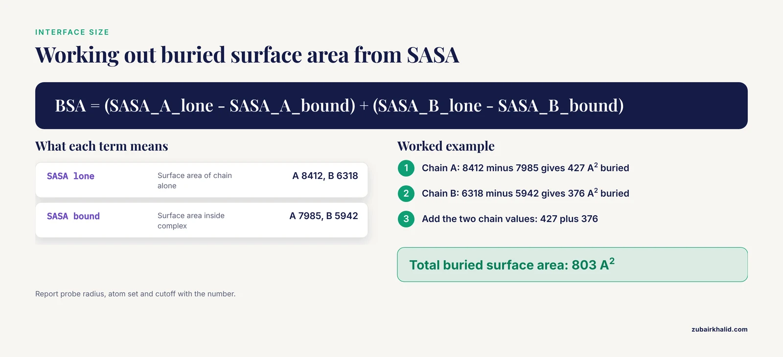
Contact counts tell you how many residues touch. Buried surface area (BSA) tells you how much solvent-exposed surface disappears when the two chains bind, which is the standard physical measure of interface size. The Shrake-Rupley algorithm, implemented in Biopython, computes solvent-accessible surface area (SASA) for the assembled complex and for each chain alone, and the difference is the buried area.
from Bio.PDB import PDBIO, PDBParser, Select
from Bio.PDB.SASA import ShrakeRupley

parser = PDBParser(QUIET=True)
structure = parser.get_structure("complex", "af2_out/ranked_0.pdb")

class KeepChain(Select):
    def __init__(self, chain_id):
        self.chain_id = chain_id
    def accept_chain(self, chain):
        return chain.id == self.chain_id

io = PDBIO()
io.set_structure(structure)
ShrakeRupley().compute(structure, level="A")

bound = {}
for chain_id in ("A", "B"):
    bound[chain_id] = sum(
        a.sasa for a in structure.get_atoms()
        if a.get_parent().get_parent().id == chain_id
    )

lone = {}
for chain_id in ("A", "B"):
    io.save(f"chain_{chain_id}.pdb", KeepChain(chain_id))
    s = parser.get_structure(chain_id, f"chain_{chain_id}.pdb")
    ShrakeRupley().compute(s, level="A")
    lone[chain_id] = sum(a.sasa for a in s.get_atoms())

for c in ("A", "B"):
    print(f"chain {c}: lone {lone[c]:.0f}, bound {bound[c]:.0f}, "
          f"buried {lone[c] - bound[c]:.0f} A^2")
print(f"total buried surface area: "
      f"{sum(lone[c] - bound[c] for c in ('A', 'B')):.0f} A^2")
Expected output:
chain A: lone 8412, bound 7985, buried 427 A^2
chain B: lone 6318, bound 5942, buried 376 A^2
total buried surface area: 803 A^2
How to interpret it: a small buried area alongside a confident-looking ipTM is a red flag consistent with the known weakness of ipTM on small interfaces [4]. The absolute size ranges associated with transient versus permanent interfaces vary by study and calculation protocol, so report your protocol (probe radius, atom set, cutoff) alongside the number rather than quoting a universal threshold.
Step 5. Ask Whether the Interface Is Confidently Predicted
This is where a purely geometric interface becomes a defensible claim. The PAE matrix tells you the expected error between every pair of residues. If the residues you found in step 3 sit in a region of mutually low PAE across the chain boundary, the model is asserting a specific, reproducible geometry. If they touch in the coordinates but sit in a high-PAE fog, the contact is essentially arbitrary.
This is the principle behind the Local Interaction Score, which was developed because ipTM alone misses interactions at small or flexible interfaces, and which derives its signal from areas of the PAE matrix with low values [4]. A practical local analysis you can run immediately restricts the PAE matrix to your interface residues:
import json
import numpy as np

with open("af2_out/ranked_0_scores.json") as handle:
    scores = json.load(handle)

pae = np.array(scores["pae"])

res_a = np.loadtxt("interface_A_vs_B.txt", usecols=0, dtype=int) - 1
res_b = np.loadtxt("interface_B_vs_A.txt", usecols=0, dtype=int) - 1

sub = pae[np.ix_(res_a, res_b)]
print("mean interface PAE:", round(sub.mean(), 2), "Angstrom")
print("max interface PAE:", round(sub.max(), 2), "Angstrom")
Expected output:
mean interface PAE: 2.14 Angstrom
max interface PAE: 7.83 Angstrom
PAE is reported in Angstrom units. A low mean with a low maximum indicates a tightly specified interface. For formal hypothesis testing at scale, use the published LIS method itself rather than a homegrown proxy, since the LIS derivation and its behavior on flexible and small interfaces were validated on large Drosophila datasets and exposed through the FlyPredictome platform [4].
Two things to check before believing a good number:
- Re-run the same calculation on all five ranked models. A real interface keeps its low interface-PAE and similar geometry across independent samples.
- Look at the PAE heatmap image (
ranked_0.pae.png) with your own eyes. A dark (low-error) block between the chain segments is the visual signature of a confident interface, and its absence disqualifies the model regardless of ipTM.
Step 6. Rank and Compare Models With Interface-Focused Scoring
AlphaFold's self-assessment scores are not the only legitimate ranker, and they are not shared across methods. VoroIF-jury is a scoring method that relies only on structural information, specifically the geometry of the subunit-subunit interface, and is therefore independent of AlphaFold self-assessment scores, which means it can rank models produced by different structure prediction methods on a common scale. A protocol combining diverse model sampling with this interface-focused scoring significantly outperformed the standard AlphaFold-Multimer pipeline in CASP15 assembly prediction [8].
The practical consequence for your analysis: when you have models from several sources, for example an AlphaFold 2 Multimer run, an AlphaFold 3 server result, and a docking refinement, rank them by interface geometry with a structure-only scorer instead of trusting any single model's self-reported confidence. This also guards against the failure mode where the model with the best ipTM has a physically implausible interface.
Practical Tips for Reliable Interface Analysis
The following tips consolidate the choices that most often determine whether an interface analysis holds up.
Sample multiple models and seeds. Because multimer predictions are stochastic, five models is a floor, not a ceiling. Interfaces that appear in only one of five samples are weak evidence.
Judge locality, not just globals. ipTM and pTM summarize the whole assembly. The published evidence shows that small or flexible interfaces can be missed by ipTM even when the interaction is real, so always pair the global score with a PAE-restricted local measure or the LIS method [4].
Use interface-focused scoring when comparing across methods. Structure-only scorers such as VoroIF-jury let you rank AlphaFold and non-AlphaFold models on one scale [8].
Diversify your inputs, not just your seeds. A proven protocol diversifies models by varying how multiple sequence alignments (MSAs) are constructed and paired and by increasing the number of recycles, then scores everything with the interface-focused scorer [8]. MSA construction remains one of the strongest levers on multimer outcome quality.
Automate interface residue extraction when scaling up. Manual residue picking does not survive a hundred pairs. AlphaPulldown provides a range of confidence scores for screening workflows [1], and AlphaPPIweb adds automated interface residue analysis directly after prediction, which removes a whole class of manual errors from ligand-receptor style screens [6].
Validate the highest-value predictions against orthogonal data. Cross-linking mass spectometry (XL-MS) captures spatial relationships between amino acid stretches in living systems. A proteome-scale workflow combining phospho-enrichable cross-linking with isobaric labeling quantified over 9,000 cross-links and loop-links and overlaid AlphaFold predictions and disorder annotations to interpret them [9]. If your predicted interface places two lysines within cross-linker reach, that is a cheap and strong consistency check.
Remember what a prediction can never establish. In the bacterial T6SS toxin study, AlphaFold 3 produced a high-confidence ternary complex with three distinct interfaces, and every one of those interfaces was then confirmed experimentally in vivo, with the key charged residues identified. That is the correct posture: the model proposes residue-level hypotheses, the experiment disposes [10].
From a Predicted Interface to Biology
Once you have a confident, well-scored interface, four directions extend the analysis into biological and therapeutic territory.
Mapping Mutations Onto the Interface
Because interface residues are identified as a concrete list, disease-associated variants can be projected onto them directly. In a study of renal cell carcinoma drivers, researchers predicted high-confidence complexes for proteins such as TCEB1, KMT2C/D, KDM6A, TSC1, and TRRAP, mapped somatic missense mutations from large genome-sequencing datasets onto predicted and experimental interfaces, and evaluated their effects on binding affinity, finding more than 100 cancer somatic mutations affecting the binding affinity of complexes formed by key drivers such as VHL and TCEB1. Interfaces such as NRF2-MAFK emerged as candidate drug-target surfaces [11]. A similar logic has been applied in plants, where rice GWAS mutations were mapped onto AlphaFold Database structures partitioned into domains, and interaction partners were modeled for proteins carrying mutations at predicted PPI sites [12].
Viral and pathogen examples show the same workflow resolving mechanism-level questions. AlphaFold 3 modeling of the monkeypox virus entry fusion complex showed that the G9 M142I mutation, an APOBEC3-type mutation associated with lineage IIb B, did not alter the folding of G9 alone but shifted the conformation of the G9/A16 subcomplex and enlarged the interfacial gap within the G9/A16/A56/K2 quaternary complex, reducing docking stability. ELISA experiments then confirmed that the mutation reduces binding affinity [2]. In every one of these cases the analytical step is identical to steps 3 through 5 above, with variant coordinates overlaid on the residue lists.
Interface Energetics and Hotspots
Interfaces are not uniformly important. Combining ribosome profiling, imaging, and molecular dynamics on co-translational assembly showed that only a few residues act as hotspots with high binding energy that anchor the entire interface assembly, and that disease missense variants disrupt these hotspot clusters [13]. For interface engineering, this means a flat per-residue contact list is only the starting point. Computing per-residue binding energy, for example with Rosetta or molecular dynamics decomposition, concentrates your mutagenesis and design effort on the handful of residues that matter, an approach also used to identify stabilizing hotspots in the SARS-CoV-2 nsp7 dimer interface [14].
Using Predicted Interfaces for Drug Discovery
AlphaFold models are now routinely used as docking targets for PPI modulation. A benchmark across eight docking protocols on sixteen interactions with validated modulators found similar performance between experimental structures and AF2 models, with local docking strategies outperforming blind docking, and molecular dynamics refinement improving outcomes for both native and AF2 models while showing significant variability across conformations [15]. So the predicted interface is a legitimate starting structure for ligand docking, provided you generate a conformational ensemble rather than docking into a single static model. The caveat about conformations extends to cofactors: a comparison of the human serum albumin to CD36 receptor interaction found that the predicted interface architecture was markedly sensitive to which fatty-acid ligand occupied albumin, and that docking and AlphaFold 3 rankings disagreed, which is a concrete warning that interface geometry can depend on ligand state [16].
Scaling to Whole Interactomes
Two lessons from large-scale studies apply to any screen. First, combining fast coevolution-based pre-screening with high-resolution modeling works: in the human mitochondrial proteome analysis, RoseTTAFold coevolution was computed for roughly 95 percent of mitochondrial protein pairs, and only top-ranked pairs proceeded to AlphaFold modeling of the complexes, which produced precise contact probabilities and interfaces for previously uncharacterized pairs [17]. Second, structure prediction can rapidly expand structural coverage of interaction networks that experiments have barely touched, as shown for human-pathogen PPIs where predictions for 9,452 interactions, of which only 10 had known structures, yielded 30 interactions with expected TM-score at or above 0.9 and were partly confirmed by native mass spectrometry [18].
Common Mistakes and Limitations
These are the errors that most frequently invalidate an AlphaFold-based interface analysis, along with their fixes.
Trusting ipTM as a binding verdict. The single most common mistake. ipTM is reflective of structural integrity but demonstrably misses physiologically relevant interactions at small interfaces or within flexible regions [4]. Fix: always compute a PAE-restricted local measure or LIS in addition to ipTM, and check the PAE heatmap visually.
Analyzing one model instead of an ensemble. Multimer sampling is stochastic, and different runs of the same pair can produce different interface placements. Fix: run at least five models, compare interfaces across them, and treat single-sample interfaces as unproven. For systematic study of how interfaces change with modeling context, use ensemble tools such as MultimerMapper [7].
Assuming the pairwise interface is the biological interface. A two-chain model cannot tell you whether that surface is occluded inside a larger assembly or whether a third partner competes for it. Interfaces and conformations vary depending on which components are included in the prediction [7]. Fix: model relevant third partners and higher-order stoichiometries before drawing conclusions about interface relevance in vivo.
Ignoring numbering mismatches when mapping mutations. A mutation that appears interfacial in UniProt numbering may be outside the modeled construct, or vice versa. Fix: keep an explicit mapping from PDB residue numbers to reference-sequence numbering, and re-derive it whenever you change the construct definition. Mutation-interface studies that skipped this step produce irreproducible affinity claims [11].
Using AlphaFold self-assessment as the only ranking criterion across methods. Self-assessment scores are not comparable between AlphaFold versions or between AlphaFold and docking or coevolution pipelines. Fix: rank cross-method model sets with a structure-only interface scorer such as VoroIF-jury, which was designed precisely for this purpose [8].
Docking into a single static predicted structure. Docking outcomes vary significantly across conformations even after MD refinement, and ensemble generation improves results [15]. Fix: dock into multiple models from multiple seeds, and prefer local docking around your known interface over blind docking.
Treating a confident interface as a confirmed one. Confidence metrics quantify how self-consistent the model is, not whether the interaction exists in the cell. Even excellent ternary predictions of toxin-immunity systems required independent biochemical and in vivo confirmation of each predicted interface [10]. Fix: plan at least one orthogonal validation, such as co-purification, cross-linking mass spectrometry [9], or binding assays, for every interface you intend to publish or act upon.
Overlooking ligand and state dependence. Interface architecture can change with the ligand state of the proteins involved, and different prediction and docking methods can disagree on the resulting geometry [16]. Fix: model the relevant liganded and unliganded states explicitly when the biology involves small-molecule carriers or occupancy-sensitive receptors.
Frequently Asked Questions
What ipTM score should I use as a cutoff for calling an interaction?
There is no universal cutoff, and relying on one alone is unsafe because ipTM can miss real interactions with small or flexible interfaces [4]. As a screen, published analyses have treated scores above roughly 0.6 as predicted binding and below 0.6 as predicted non-binding, with confident binders in the 0.77 to 0.82 range [5]. Confirm borderline cases with a PAE-based local analysis and multiple sampled models.
Can I trust a high-confidence AlphaFold interface without experimental validation?
Treat it as a precise, testable hypothesis rather than a result. Predicted interfaces have been confirmed experimentally in several studies, but only after orthogonal assays were run, including in vivo interaction tests and binding measurements that validated each predicted interface and its key residues [10]. Cross-linking mass spectrometry provides another independent consistency check at proteome scale [9].
What is the difference between pTM and ipTM?
pTM measures predicted accuracy of the overall multi-chain topology, while ipTM (interface predicted TM-score) measures the same quantity restricted to residues that span chain boundaries. ipTM is therefore the more relevant global screen for interactions, but it summarizes the whole interface and says nothing about which specific residues contact each other, which is what the PAE matrix provides.
How do I find interface residues from an AlphaFold PDB file?
Compute all heavy-atom pairs between different chains and keep those within a short distance cutoff, commonly around 4.5 Angstroms. The Biopython and SciPy script in step 3 does this and writes per-chain residue lists. Web platforms such as AlphaPPIweb automate the same interface residue extraction directly after structure prediction [6].
Should I use AlphaFold 2 Multimer or AlphaFold 3 for interface analysis?
AlphaFold 3 showed the best overall PPI interface prediction performance in a recent benchmark of cofolding methods that included Boltz-1, Chai-1, Protenix, and RoseTTAFold All-Atom [3], which makes it a strong default through the AlphaFold server for small jobs. AlphaFold 2 Multimer through local pipelines remains the workhorse for high-throughput screens, and both benefit from interface-focused, structure-only scoring when compared head to head [8].
Why does the same protein pair give different interfaces in different predictions?
Because multimer predictions are stochastic and because interface geometry depends on modeling context, meaning which other chains are present in the prediction. Ensemble analysis with tools such as MultimerMapper is designed to reveal these alternative interaction modes statistically and to infer stoichiometry from prediction ensembles [7]. Reproducibility of an interface across seeds and contexts is itself evidence for it.
How can I analyze many protein pairs at once instead of one at a time?
Use a screening package. AlphaPulldown streamlines PPI screens and higher-order oligomer modeling on top of AlphaFold-Multimer with a command-line interface, multiple confidence scores, and a graphical analysis tool [1]. For a browser-based alternative with automated interface residue analysis and bait-versus-candidate screening, AlphaPPIweb wraps the same prediction engine [6].
Can AlphaFold structures be used to dock small molecules at protein-protein interfaces?
Yes. A benchmark of eight docking protocols found similar performance between AF2 models and experimentally solved structures, with local docking outperforming blind docking and molecular dynamics refinement helping in some cases [15]. The main caveat is conformational variability, so build an ensemble of predicted and refined structures rather than docking into one static model.
Sources
- AlphaPulldown-a python package for protein-protein interaction screens using AlphaFold-Multimer.
- Structural Insights into the Impact of the M142I Mutation in Monkeypox Virus G9 Protein on Subcomplex Formation Revealed by AlphaFold 3 Modeling.
- Benchmarking Cofolding Methods for Molecular Glue Ternary Structure Prediction.
- Enhanced Protein-Protein Interaction Discovery via AlphaFold-Multimer.
- Predicted protein-protein interactions between sugar beet root maggot trypsins and sugar beet Kunitz trypsin inhibitors using deep learning.
- AlphaPPIweb: an integration platform for protein-protein interaction prediction and evaluation.
- Context-dependent protein structure prediction analysis and complex stoichiometry inference with MultimerMapper.
- Prediction of protein assemblies by structure sampling followed by interface-focused scoring.
- PhoXplex: Combining Phospho-enrichable Cross-Linking with Isobaric Labeling for Quantitative Proteome-Wide Mapping of Protein Interfaces.
- "Molecular insights into the bactericidal toxin Tle1 of Pseudomonas aeruginosa: Interaction with VgrG, its adaptor, and its immunity protein".
- Computational analysis of protein-protein interactions of cancer drivers in renal cell carcinoma.
- Employing AlphaFold and TED to explore the structural impacts of stress-associated mutations in rice.
- Diverging co-translational protein complex assembly pathways are governed by interface energy distribution.
- Interface design of SARS-CoV-2 symmetrical nsp7 dimer and machine learning-guided nsp7 sequence prediction reveals physicochemical properties and hotspots for nsp7 stability, adaptation, and therapeutic design.
- Evaluating ligand docking methods for drugging protein-protein interfaces: insights from AlphaFold2 and molecular dynamics refinement.
- Molecular Mechanisms of Interaction of Human Serum Albumin with the CD36 Receptor: Insights from Molecular Dynamics Simulations.
- Human mitochondrial protein complexes revealed by large-scale coevolution analysis and deep learning-based structure modeling.
- AI-first structural identification of pathogenic protein target interfaces.