AlphaFold for Non-Model Organisms

By Dr. Zubair Khalid, DVM, MS, PhD · 2026-11-11

Most AlphaFold guides quietly assume you work on human, mouse, or E. coli. If you study a coral, a parasite, a crop pathogen, or an animal with no genome project, the workflow changes in ways that decide whether your prediction is useful or quietly wrong. By the end of this article you will be able to check whether your protein already has a structure in the AlphaFold Protein Structure Database, fetch a clean sequence, run a prediction with the AlphaFold Server or ColabFold, read the confidence metrics correctly, and recognize the failure modes that hit non-model organisms hardest.

Here is what you need on hand before you start:

• A protein sequence in FASTA format, either from your own sequencing data or from a database such as UniProt or NCBI Protein.
• A Google account if you want to use the AlphaFold Server or the free ColabFold notebook. Both run in the browser with no installation.
• Python 3.9 or newer and either Google Colab or a Linux machine with an NVIDIA GPU if you want to run predictions yourself.
• Roughly 30 minutes for a first prediction using the server route, or 1 to 2 hours for the local ColabFold route including installation.

This guide covers AlphaFold 2 and AlphaFold 3, the AlphaFold Server, and ColabFold. The step by step walkthrough uses a real worked example throughout so you can compare your output against mine.

Why Non-Model Proteins Are Harder for AlphaFold

AlphaFold 2, published by DeepMind in Nature in 2021, predicts a protein's three dimensional structure from its amino acid sequence. The core input is a multiple sequence alignment (MSA), which is the list of related sequences found in databases and stacked against your query. Residues that evolve together leave co-evolutionary signals in that alignment, and the network uses those signals to infer which residues are neighbors in three dimensions.

The quality of the MSA is therefore the single biggest variable in prediction quality. This is exactly where non-model organisms suffer. AlphaFold's training and its default database searches lean heavily on UniRef, a comprehensive sequence database maintained by UniProt, and on metagenomic databases such as BFD and MGnify that contribute hundreds of millions of additional sequences. A human kinase sits inside an alignment of tens of thousands of homologs. A protein from an under-sequenced fungus, a rare parasite, or a newly described bacterium may find only a few dozen homologs, and some orphan proteins find almost none at all.

Two consequences follow. First, per-residue confidence drops, especially for regions with no detectable homology. Second, and more dangerous, a shallow alignment can push the network toward a plausible-looking but wrong fold, because the model has no strong evidence for the correct one and falls back on patterns learned from distant relatives. A prediction with a confident-looking ribbon diagram and a low global score is the classic trap for anyone working on non-model organisms. You will learn to detect it in Step 5.

There is also good news. Since 2022, DeepMind and EMBL's European Bioinformatics Institute (EMBL-EBI) have released predicted structures for nearly every protein in the UniProt knowledgebase, more than 200 million of them, through the AlphaFold Protein Structure Database (AFDB). Most proteomes from non-model organisms with a reference genome are already in there. Your first task, before any prediction, is to check whether you need to run AlphaFold at all.

Start Here: Check AlphaFold DB Before You Predict Anything

Search AFDB at alphafold.ebi.ac.uk by UniProt accession, protein name, or organism name. If your organism's proteome was available in UniProt when the database was built, its structures exist already, and downloading them beats predicting them.

If you have a UniProt accession, you can also fetch the structure file directly over HTTPS. The green fluorescent protein from the jellyfish Aequorea victoria, an organism most people would call non-model, carries accession P42212 in UniProt. The predicted structure downloads like this:

curl -s -o AF-P42212-F1-model_v4.pdb \
  "https://alphafold.ebi.ac.uk/files/AF-P42212-F1-model_v4.pdb"
head -2 AF-P42212-F1-model_v4.pdb

Expected output:

ATOM    835  N   GLY A   1      -5.250  3.501  -5.105  1.00 85.42           N
ATOM    836  CA  GLY A   1      -5.058  3.310  -3.948  1.00 88.75           C

The number in the last numeric column before the element symbol is the per-residue pLDDT score stored in the B-factor field, which you will learn to read in Step 5.

Three practical points about AFDB for non-model organisms:

1. Coverage follows UniProt. If your species has proteome entries in UniProt, AFDB likely has its predicted structures. If you only have a draft genome or transcriptome with no UniProt entries, nothing exists yet and you must predict yourself.
2. Version matters. Files are versioned (v1, v2, v3, v4). When you compare a model against your own prediction or against experimental data, note which version you downloaded because newer versions can differ.
3. AFDB models are single chains with no ligands, no cofactors, and no partner chains. A membrane receptor in AFDB is missing its lipid environment and any bound ions.

If your protein is not in AFDB, continue to the walkthrough.

The AlphaFold Server: Fastest Route for Small Jobs

The AlphaFold Server, launched in May 2024 by Google DeepMind, is a free web interface to AlphaFold 3. It accepts proteins, DNA, RNA, ions, ligands, and chemical modifications, which makes it dramatically more useful than AlphaFold 2 for non-model organisms where your protein may bind a metal, a heme, or an unusual cofactor. According to Google DeepMind's AlphaFold Server documentation, jobs are limited to 20 per day and to 10,000 total tokens, where a token counts roughly as one residue or one atom-scale component.

The server route takes about five minutes of hands-on time:

1. Go to alphafoldserver.com and sign in with a Google account.
2. Click "New Job" and paste your protein sequence, or click "Add Entity" and choose the molecule type. Paste FASTA or raw sequence, either works.
3. Add any partner molecules: a second protein chain, a DNA strand, ATP, a metal ion, or a small molecule by name or SMILES string.
4. Click "Submit" and wait. Typical jobs finish in minutes to a few hours depending on queue load.
5. Download the results as an mmCIF file containing the predicted structure and an error-rate (PAE) matrix.

The server's strengths for non-model organisms are its ability to include ligands and its ability to model complexes up to the token limit. Its limits are the daily job quota, the token ceiling, no control over MSA settings, and a terms of service that restricts output to non-commercial use. For a survey of many proteins, or for anything needing custom MSA handling, use ColabFold instead.

AlphaFold Non-Model Organisms Tutorial, Step by Step

This is the core walkthrough. It uses ColabFold, an open-source reimagination of AlphaFold 2 developed by the Kim lab at Seoul National University and collaborators, because it gives you control over the MSA, runs on free Google Colab GPUs, and prints the diagnostics you need to diagnose weak predictions. Every command below runs either in a Colab notebook or in a local terminal.

Step 1: Fetch and Clean the Sequence

Start from the right sequence, because everything downstream depends on it. Pull it from UniProt with a single command:

curl -s "https://rest.uniprot.org/uniprotkb/P42212.fasta" > query.fasta
cat query.fasta

Expected output:

>sp|P42212|GFP_AEQVI Green fluorescent protein OS=Aequorea victoria OX=6100 GN=gfp PE=1 SV=1
MSKGEELFTGVVPILVELDGDVNGHKFSVSGEGEGDATYGKLTLKFICTTGKLPVPWPTLVTTF
TTYGVQCFSRYPDHMKQHDFFKSAMPEGYVQERTISFKDDGTYKTRAEVKFEGDTLVNRIELKG
IDFKEDGNILGHKLEYNYNSHNVYIMADKQKNGIKVNFKIRHNIEDGSVQLADHYQQNTPIGDG
PVLLPDNHYLSTQSALSKDPNEKRDHMVLLEFVTAAGITHGMDELYK

Now clean it. Each of these checks prevents a specific downstream failure:

1. Strip stop codons and asterisks. An asterisk inside the sequence breaks some parsers with the message ValueError: Invalid FASTA sequence or silently truncates the model.
2. Decide what to do about low-complexity and disordered tails. Long disordered tails consume compute and always score poorly. You can predict the full length once, then re-run the ordered core alone for cleaner models.
3. Resolve isoform numbering. If the transcript you sequenced differs from the UniProt canonical isoform, note every difference now. Mapping a mutation onto the wrong isoform numbering is a classic downstream error.
4. Split multi-domain proteins longer than about 2,700 residues. AlphaFold 2 runs into memory limits on very long chains. Predict each domain separately, using domain boundaries from a tool such as InterPro or from your own homology search.

If your protein comes from a genome you assembled yourself, run one round of quality control first. Search the sequence against the NCBI nr database with BLASTP to confirm it is what you think it is, and check for frameshift artifacts near assembly gaps. Predicting a frameshifted sequence produces a structure that looks fine and means nothing.

Step 2: Install ColabFold

The fastest path is the ColabFold notebook hosted on Google Colab, which requires no installation at all. Search "ColabFold AlphaFold2" on Google Colab, open the notebook, and follow its cells. If you prefer a local install on Linux with an NVIDIA GPU, install through pip:

conda create -n colabfold python=3.9 -y
conda activate colabfold
pip install "colabfold[batch]"
colabfold_batch --help | head -20

Expected output ends with a long usage block beginning:

Usage: colabfold_batch [OPTIONS] INPUT OUTPUT_DIR

If pip fails during JAX installation, pin a JAX version that matches your CUDA toolkit. The error usually looks like ERROR: No matching distribution found for jax[cuda12]==... and the fix is documented in the ColabFold README, which lists supported CUDA versions. Verify your driver with nvidia-smi before pinning anything.

Step 3: Run the Prediction

A first pass for a single-chain protein from a non-model organism should look like this:

colabfold_batch \
  --model-type alphafold2_ptm \
  --num-models 5 \
  --num-recycle 3 \
  --msa-mode mmseqs2_uniref_env \
  query.fasta results/

The console prints progress for each stage, MSA generation first, then model inference. A successful run ends with lines like these (your exact numbers will differ):

2026-01-15 14:02:11,037 Running model_1
2026-01-15 14:02:41,227 rank_001_alphafold2_ptm_model_1 pLDDT=91.7 pTM=0.92
2026-01-15 14:02:41,228 rank_002_alphafold2_ptm_model_1 pLDDT=91.2 pTM=0.91
...
Done in 890.3s

A pLDDT above 90 and a pTM above 0.9 on a first pass tells you the MSA was deep enough and you can move to interpretation. If your numbers come out far lower, keep going to Step 6, which is written specifically for that situation.

The flags that matter most for non-model organisms are collected in this table:

Step 4: Read the Output Files

The results directory contains everything you need:

ls results/ | head -12

query_2c0f4MSA_coverage.png
query_2c0f4MSA_depth.png
query_2c0f4PAE.png
query_2c0f4_unrelaxed_rank_001_alphafold2_ptm_model_1.pdb
query_2c0f4_unrelaxed_rank_002_alphafold2_ptm_model_1.pdb
query_2c0f4_relaxed_rank_001_alphafold2_ptm_model_1.pdb
query_2c0f4_rank_001_alphafold2_ptm_model_1_scores.json
query_2c0f4_rank_001_alphafold2_ptm_model_1_Scores_and_pLDDT.png
query_2c0f4_plddt_rank_001_alphafold2_ptm_model_1.png

What each file is for:

1. The unrelaxed PDB files are the raw network outputs. The relaxed versions have gone through a short Amber energy minimization and are what you should use for visualization and downstream work.
2. The _scores.json file holds the headline numbers: pLDDT, pTM, and, for complexes, ipTM. Print it with python -m json.tool and look at max_ptm, iptm, and plddt.
3. The MSA coverage and depth plots show how many homologs were found and how completely they cover your query. A coverage plot with a big gap across some region means the model had almost no co-evolutionary information there, which predicts low confidence in exactly that region.
4. The PAE plot is the predicted aligned error matrix, and it is the most informative single image in the folder. Read it in Step 5.

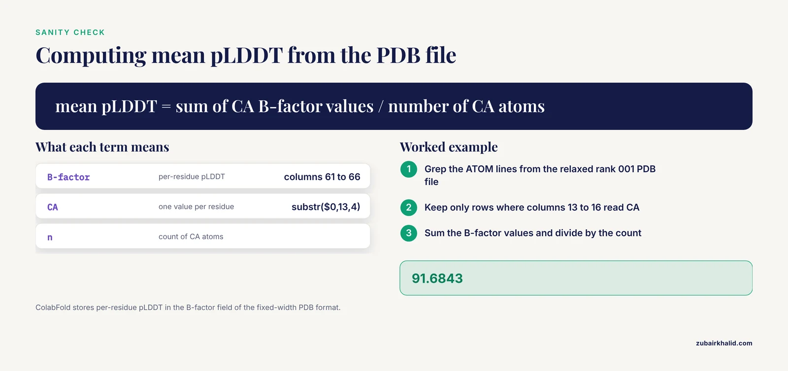
Compute the mean pLDDT yourself from the PDB to sanity check the console summary:

grep "^ATOM" results/query_2c0f4_relaxed_rank_001_alphafold2_ptm_model_1.pdb \
  | awk 'substr($0,13,4)==" CA " {s+=substr($0,61,6); n++} END {print s/n}'

Expected output:

91.6843

This works because ColabFold stores the per-residue pLDDT in the B-factor column, columns 61 through 66 of the fixed-width PDB format.

Step 5: Judge the Confidence

AlphaFold reports confidence through three related metrics. Understanding all three, and their limits, is what separates a useful prediction from a pretty picture.

pLDDT is the per-residue predicted local distance difference test score, expressed on a scale of 0 to 100. It estimates how well each residue's position matches a reference measurement. Per the AlphaFold DB documentation at EMBL-EBI, the standard color bands are: above 90, very high confidence and backbone accuracy; between 70 and 90, backbone generally correct with side chains uncertain; between 50 and 70, low confidence and unreliable local geometry; below 50, very low confidence, typically intrinsically disordered regions. Two habits to build immediately. First, never average pLDDT across a protein with one ordered domain and one disordered tail, because the average hides which half is trustworthy. Second, treat anything below 50 as information, not failure, because it often correctly flags disorder.

PAE is the predicted aligned error, measured in angstroms, between every pair of residues. Low PAE within a domain and low PAE between two domains means the relative placement of those domains is well determined. High PAE between two domains means the model knows each domain's shape but is guessing how they connect. For non-model organisms this distinction matters enormously, because a shallow MSA often supports one domain confidently while the inter-domain arrangement stays random. When you see a PAE matrix with dark intra-domain blocks and bright inter-domain blocks, cut the protein at the domain boundary and treat the arrangement as undetermined.

pTM and ipTM are global and interface level estimates of structural similarity to the true structure, on a scale of 0 to 1. For complexes predicted with the multimer model, the AlphaFold-Multimer authors report that an ipTM above roughly 0.8 usually indicates a correctly predicted interface, and values below that range deserve suspicion. A complex can score beautifully on pLDDT while the subunits float in the wrong relative orientation, which is why ipTM, not pLDDT, is the number to check first for any multi-chain job.

One additional check that catches shallow-MSA failures: run the same sequence twice with different random seeds by adding -num-seeds 2. If the two runs produce topologically different folds, the prediction is not settled and no amount of manual inspection will rescue it. Agreement across seeds and across the five default models is the strongest cheap evidence you have.

Step 6: Fix a Weak Prediction

When pLDDT comes back low and the PAE matrix looks noisy, work through these options in order, because they are ordered by how often they help:

1. Deepen the MSA locally. ColabFold's default searches UniRef and environmental databases through the MMseqs2 web API. If your organism belongs to an under-sampled clade, build your own MSA with jackhmmer against UniRef100 or against a taxonomic slice relevant to your organism, then supply it with -msa-mode custom. Custom MSAs are built with the A3M format, and ColabFold documents the converter script for turning standard FASTA alignments into A3M.
2. Add orthologs deliberately. A shallow alignment can often be rescued by including homologs from closely related species that standard searches miss because they hit only over a short fragment. Run a sensitive search with a tool such as HMMER's hmmsearch against a profile built from your initial hits.
3. Reduce MSA diversity rather than increase it. If the alignment contains many distant, noisy relatives, capping the depth with -max-msa 16:32 sometimes sharpens the co-evolutionary signal enough to change the answer. This tip comes from the ColabFold documentation and repeatedly rescues difficult cases.
4. Turn templates off or on. For a non-model protein whose fold is unusual for its family, a template from a distant homolog can drag the model into a wrong state. Conversely, a good template can carry a prediction when the MSA is thin. Test both settings and compare PAE matrices.
5. Switch to AlphaFold 3 for ligand problems. If the weak region is a binding site whose geometry depends on a cofactor, model the protein with its ligand through the AlphaFold Server. AlphaFold 3 was trained on complexes and often resolves local geometry that ligand-free AlphaFold 2 leaves uncertain.
6. Accept the result. Some orphan proteins, particularly rapidly evolving secreted effectors from pathogens, have no detectable homologs at all. For these, run in single-sequence mode, interpret only the well-structured core, and plan an experimental structure determination.

Running Full AlphaFold 2 on Your Own Hardware

When you need hundreds of predictions, such as a whole pathway from a newly sequenced organism, the command line version of AlphaFold 2 from the DeepMind repository is more efficient than repeated ColabFold runs, because you keep the reference databases local. The tradeoff is disk and memory. Per the AlphaFold repository documentation, the full database set includes BFD at roughly 1.8 terabytes, and the total download runs to a couple of terabytes with search indexes. The reduced database preset substitutes smaller MSA sources and fits into a few hundred gigabytes of disk with a machine memory budget in the hundreds of gigabytes for search.

The core sequence of commands:

git clone https://github.com/google-deepmind/alphafold.git
cd alphafold
# Download databases (one-time, several hours to days)
scripts/download_all_data.sh /data/alphafold_dbs
# Run a prediction
python3 run_alphafold.py \
  --fasta_paths=query.fasta \
  --output_dir=results \
  --data_dir=/data/alphafold_dbs \
  --db_preset=full_dbs \
  --model_preset=monomer \
  --max_template_date=2026-01-01

The -max_template_date flag deserves one sentence of explanation: it excludes structural templates released after the given date, and it exists so that benchmarking experiments are fair. For routine prediction on your own protein, set it to the present.

For most non-model organism projects, the reduced database preset plus a single A100-class GPU is the practical entry point, and the DeepMind documentation describes the hardware requirements for each preset. If your institution lacks such hardware, ColabFold on Colab or on a rented cloud GPU remains the better route, because the reference databases stay hosted.

AlphaFold 3, whose code DeepMind released through GitHub in late 2024 under the name alphafold3, handles proteins, nucleic acids, ligands, and modifications within one network. Its model parameters are not a direct download. Google requires an approved request form for the weights, and the terms distinguish academic and commercial uses, so read the current terms on the repository before planning a pipeline around it.

Common Mistakes and Limitations

These are the errors that cost non-model organism researchers the most time, listed with the symptom you will see and the fix.

1. Treating a low pLDDT region as a prediction failure. Intrinsically disordered regions score below 50 by design because AlphaFold predicts one conformation and disorder means many conformations. Trim them from your models rather than debugging them.
2. Reading pLDDT as evidence for domain arrangement. pLDDT says nothing about whether two domains sit in the right relative positions. Only the PAE matrix answers that. A model can have mean pLDDT of 90 and a completely wrong inter-domain orientation.
3. Predicting single chains when the protein works as a complex. A homodimer predicted as a monomer can bury the wrong face of the chain. ColabFold handles this with -model-type alphafold2_multimer_v3 and separate FASTA headers per chain. Check for known oligomerization state in homologs before choosing.
4. Trust the fold, distrust the details. AlphaFold's side-chain geometry in low confidence regions is unreliable, and loop conformations near functional sites can be off by angstroms even at high confidence. Do not design point mutations against a loop with pLDDT of 65.
5. Forgetting that the prediction is a static structure. AlphaFold outputs one conformation, usually close to the dominant state seen in homologs. Proteins known to undergo large conformational changes, such as transporters and some kinases, may be predicted in whichever state the templates and MSA favor, and no flag forces the alternate state.
6. Comparing a fragment prediction to a full-length experimental structure. If you modeled only the kinase domain but compare to full-length PDB entries, RMSD values will be inflated for reasons that have nothing to do with model quality. Match the residues you modeled.
7. Ignoring isoform numbering. Non-model organisms often have annotation pipelines with multiple gene models. If your residue numbering comes from a transcript while your prediction used a UniProt canonical isoform, every residue-labeled claim you make can be off by an insertion somewhere in the middle. Align the two sequences once and record the offset.
8. Skipping contamination checks on custom MSAs. If you build your own MSA from a draft genome, a few contaminant sequences or duplicated near-identical copies can dominate the alignment. Deduplicate at a reasonable sequence identity threshold and inspect the alignment visually before trusting a prediction built on it.
9. Losing work on free Colab. Free Colab sessions disconnect after a period of inactivity and time out after about 12 hours. Save your result directory to Google Drive immediately after each batch finishes, because a disconnected session takes the outputs with it.
10. Over-interpreting a single beautiful model. For any result that will drive experiments, demand agreement across seeds and across the five models, a clean PAE matrix, and a sensible comparison to at least one distant homolog's experimental structure. One model from one seed is a hypothesis.

A final limitation that deserves its own sentence: AlphaFold predicts structure from sequence alone and knows nothing about your organism's biology, so experimental validation remains necessary for any individual result that matters.

Frequently Asked Questions

Can AlphaFold predict structures for proteins with no known homologs?

Sometimes, but the confidence is usually low. AlphaFold 2 relies heavily on the multiple sequence alignment, so orphan proteins from non-model organisms often produce models with confident local fragments and uncertain global topology. Run a prediction with single-sequence mode to see what the model infers from the sequence alone, then treat the well-scored core as a hypothesis.

Is the AlphaFold Server free to use?

Yes. Google DeepMind provides the AlphaFold Server free of charge with a daily job quota of 20 jobs and a limit of 10,000 tokens per job, and the terms of service restrict use to non-commercial purposes. For commercial work, or for jobs beyond the token limit, you need local AlphaFold or ColabFold.

How long a sequence can AlphaFold handle?

AlphaFold 2 runs into GPU memory limits on chains much longer than about 2,700 residues. The practical fix is to predict long proteins as separate domains using boundaries from a domain annotation resource, then dock or stitch the results with the PAE matrix as your guide.

What does pLDDT mean?

pLDDT is a per-residue confidence score from 0 to 100 that estimates how accurately the model places each residue. Per EMBL-EBI's AlphaFold DB documentation, scores above 90 indicate very high accuracy, 70 to 90 confident backbone with uncertain side chains, 50 to 70 low confidence, and below 50 very low confidence, often marking disorder.

How do I know if my protein already has a predicted structure?

Search the AlphaFold Protein Structure Database at alphafold.ebi.ac.uk by UniProt accession, gene name, or organism. If your organism's proteome exists in UniProt, its predictions are almost certainly already available for direct download, which saves you an entire prediction run.

Can AlphaFold predict protein complexes?

Yes, in two ways. AlphaFold 2's multimer mode, available in ColabFold through the alphafold2_multimer_v3 model type, handles multi-chain complexes, and AlphaFold 3 on the AlphaFold Server handles proteins together with nucleic acids, ions, and ligands. For complexes, judge quality by the ipTM score rather than pLDDT, with values above roughly 0.8 suggesting a correct interface.

Should I use AlphaFold 2 or AlphaFold 3 for my protein?

Use AlphaFold 3 when ligands, DNA, RNA, or modifications matter and your complex fits the server's token limit. Use AlphaFold 2 through ColabFold when you need custom MSA control, high throughput, or full reproducibility, because it gives you access to every MSA and model setting.

How long does one prediction take?

Through the AlphaFold Server, minutes to a few hours depending on queue load. Through ColabFold on a free Colab GPU, a typical 300-residue protein with five models and three recycles finishes in roughly 10 to 30 minutes, while long or difficult proteins and deeper MSA settings stretch that to several hours.