Using AlphaFold Models for Molecular Replacement: A Guide
By Dr. Zubair Khalid, DVM, MS, PhD ·
Molecular replacement (MR) is the crystallographic method that solves the phase problem by placing a known 3D model of your protein into the unit cell, so the measured diffraction amplitudes can be converted into an electron density map. Before AlphaFold, the quality of that starting model was the limiting factor for most difficult structures. Now a deep learning prediction, run in minutes or downloaded in seconds, is often the best model you have.
By the end of this guide you will be able to take an AlphaFold prediction from the AlphaFold server, the AlphaFold Protein Structure Database, or your own ColabFold run, prune it intelligently based on its confidence scores, split it into domains where needed, and feed it to molecular replacement in Phenix. You will also know how to judge the result and how to recover when the first attempt fails.
Here is what you need on hand before starting:
- A diffraction dataset reduced to structure factor amplitudes, typically an MTZ file with a free R flag set.
- The amino acid sequence of the construct you actually crystallized, including any expression tags, because predicted models are built from database sequences that may differ.
- A Phenix installation (Phenix includes Phaser,
phenix.process_predicted_model, and refinement tools). - Optionally, ColabFold or a local AlphaFold installation if your sequence is not already in the AlphaFold Protein Structure Database.
Why AlphaFold Models Changed Molecular Replacement
Traditional MR searches used homologous structures from the Protein Data Bank (PDB), the public archive of experimentally determined structures. When the closest homolog shared only 20 to 30 percent sequence identity, the model was often too inaccurate for the rotation and translation searches to find a clear signal, and the project stalled.
AlphaFold predictions change this in three ways:
- Coverage. A prediction covers the entire target sequence, including loops and termini that had no homologous experimental structure.
- Accuracy. For most folded regions, the predicted backbone sits within about 1 to 2 Å rmsd of the experimentally determined structure. That is comparable to a homologous model at high sequence identity.
- Self-reported confidence. Every residue carries a predicted local distance difference test (pLDDT) score on a 0 to 100 scale, and the model carries a predicted aligned error (PAE) matrix describing how confident the network is about the relative positions of each pair of residues. These scores tell you exactly which parts of the model to trust, which to prune, and how domains are arranged relative to each other [1].
The practical consequence, documented across many test cases, is that large parts of an AlphaFold model typically approach the accuracy of experimentally determined structures, while local errors and errors in the relative orientations of domains remain common and must be handled during preparation and refinement [1].
Reading the Confidence Metrics Before You Touch a Command
Two metrics drive every preparation decision.
pLDDT (predicted local distance difference test). A per-residue score from 0 to 100 stored in the B-factor column of the output file. The conventional interpretation bands, which are also the color bands used by the AlphaFold database viewer, are:
| pLDDT range | Interpretation | Typical action for MR |
|---|---|---|
| Above 90 | Very high confidence, backbone usually accurate to better than 1 Å | Keep |
| 70 to 90 | Confident, well-modeled backbone | Keep, refine normally |
| 50 to 70 | Low confidence, backbone approximate | Keep only with caution or prune |
| Below 50 | Very low confidence, likely disordered or wrong | Prune or split around |
PAE (predicted aligned error). A matrix giving the expected positional error in Ångströms for every pair of residues if the model were aligned on each one. Low PAE values between two regions mean the network is confident about their relative orientation. High PAE values between two regions mean the domain arrangement is a guess, even if each domain itself is individually well predicted.
The PAE matrix is the single most informative plot for MR preparation. A well-separated block structure with high inter-domain PAE tells you that placing the domains independently during MR is the correct strategy, while a single low-PAE block tells you the full-length model is safe to use as one rigid body [1].
AlphaFold Molecular Replacement Preparation: Step by Step
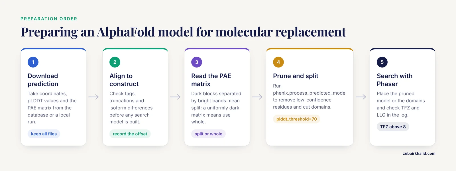
The following walkthrough covers the standard pipeline. Exact keyword names can shift slightly between Phenix versions, so when in doubt run any Phenix command with -show-defaults to list the current options.
Step 1. Obtain a prediction
If your target sequence is already in the database, download the monomer model and its PAE matrix from the AlphaFold Protein Structure Database at alphafold.ebi.ac.uk, which is operated with EMBL-EBI. If the database lacks your sequence, or you want a complex rather than a single chain, use the AlphaFold server hosted by Google DeepMind, which accepts up to a limited number of chains and returns predicted complexes, or run a local prediction.
A typical ColabFold invocation looks like this:
colabfold_batch --msa-mode server target_seq.fasta ./af_outputThe output directory contains the coordinates (usually in mmCIF format), the per-residue pLDDT values, and a PAE matrix image plus its raw values. Keep all of these files. The pLDDT scores are written into the B-factor column of the coordinate file, so downstream Phenix tools can read them directly.
Step 2. Align the predicted sequence to your crystallized construct
Predictions are built from the database or input sequence. Your construct may differ: cloning artifacts, affinity tags, missing signal peptides, or isoform mismatches. Check the alignment before anything else, because an unmodeled tag left in the MR search model wastes search volume and can degrade the signal.
A quick sequence check with Biopython:
from Bio import SeqIO
af_seq = str(next(SeqIO.parse("af_output/target_seq.fasta", "fasta")).seq)
construct = str(next(SeqIO.parse("construct.fasta", "fasta")).seq)
print(len(af_seq), len(construct))
for i, (a, b) in enumerate(zip(af_seq, construct)):
    if a != b:
        print(i + 1, a, b)
If the construct is a truncated version of the prediction, note the residue range you crystallized. You will restrict the search model to that range later.
Step 3. Inspect the PAE matrix and decide on domains
Open the PAE matrix image. Ask two questions:
- Are there off-diagonal blocks of low PAE separated by high-PAE bands? Those blocks are confidently predicted domains whose relative orientation is uncertain. Plan to split.
- Is the whole matrix dark (low PAE)? The full-length model is a valid rigid body. Plan to use it whole.
This single decision, made from data the prediction provides, is what separates efficient AlphaFold-based MR from frustrating trial and error [1].
Step 4. Prune and split with phenix.process_predicted_model
phenix.process_predicted_model is the Phenix tool built specifically for this purpose. It removes low-confidence residues and can break the model into confidently predicted domains, producing search models ready for molecular replacement or cryo-EM docking [1].
A typical run on a model where the PAE matrix suggests two domains:
phenix.process_predicted_model \
  model=af_output/ranked_0.pdb \
  plddt_threshold=70 \
  split_by_pae=True \
  pa_cutoff=8 \
  minimum_domain_length=15
Representative console output (file names and residue counts vary with your model):
Working with input model: ranked_0.pdb
Model contains 1 chain with 312 residues
Total residues removed: 41  (pLDDT below threshold 70)
Segments remaining: 2
  Segment 1: residues 1-148, mean pLDDT 93.4
  Segment 2: residues 157-301, mean pLDDT 91.2
Writing processed model to: ranked_0_processed.pdb
Writing domain 1 to: ranked_0_processed_domain_1.pdb
Writing domain 2 to: ranked_0_processed_domain_2.pdb
The key options are summarized in the table below.
| Option | What it does | Practical guidance |
|---|---|---|
plddt_threshold | Residues below this pLDDT are removed | 70 is the standard starting value, raise it for stubborn cases |
split_by_pae | Uses the PAE matrix to cut the model into domains | Turn on when the PAE matrix shows separated blocks |
pa_cutoff | PAE value (in Å) used to decide whether two regions belong to one domain | Smaller values split more aggressively |
minimum_domain_length | Smallest fragment kept as a domain | Prevents tiny unreliable fragments from cluttering the MR search |
remove_low_confidence_segments | Deletes short low-confidence stretches rather than trimming the ends | Useful for cleaning internal uncertainty |
The pruned pLDDT values remain in the B-factor column of the output files, which matters later for refinement weighting.
Step 5. Run molecular replacement with Phaser
Phaser, distributed inside Phenix, performs the rotation and translation searches and returns likelihood-based scores. You can run it from the Phenix GUI (Molecular Replacement, then supply the MTZ file, sequence file, and search model files) or from the command line. A minimal automated run with phenix.automr:
phenix.automr \
  data=data.mtz \
  model=ranked_0_processed.pdb \
  sequence_file=construct.fasta
For a manually controlled search with split domains, run Phaser once per domain or supply the domains as an ensemble. A simple Phaser-style invocation through Phenix looks like this:
phenix.phaser \
  data=data.mtz \
  model=ranked_0_processed_domain_1.pdb \
  sequence_file=construct.fasta
Check the log for two numbers:
- TFZ (translation-function Z score). Values above roughly 8 usually indicate a correct placement, values between 5 and 8 are ambiguous, and values below 5 usually mean the search failed.
- LLG (log-likelihood gain). Higher is better, and it should increase when the second domain is placed after the first.
A correct solution places the domains in a chemically sensible arrangement with no severe steric clashes at crystallographic symmetry contacts.
Step 6. Refine and rebuild, keeping the prediction as a restraint
An MR solution built on a predicted model inherits the model's errors, and naive refinement can amplify model bias, where the map is distorted toward the starting model. Two practices reduce this risk.
First, run refinement with the prediction as an external reference restraint, so well-predicted regions stay put while genuinely wrong regions can move:
phenix.refine data.mtz refined_model.pdb \
  reference_model.enabled=True \
  reference_model.reference=af_output/ranked_0.pdb
Second, use the pLDDT values carried in the B-factor column to modulate local restraints, and rebuild by hand in a tool such as Coot or ISOLDE. ISOLDE, the interactive molecular-dynamics-based rebuilding tool in ChimeraX, uses these same confidence metrics to weight torsion and atom-atom distance restraints, which lets you rearrange the complete AlphaFold model to match the placed fragments and substantially reduces the amount of manual rebuilding of connecting regions [1].
Handling the Hard Cases: Multimers, Multi-Helical Targets, and Very Large Assemblies
Some targets resist the standard pipeline. Multi-helical proteins, multimeric complexes, and extremely large structures can fail MR even with a good prediction, because a single error in a long model propagates through the whole placement.
A published strategy from 2024 addresses exactly this situation. It combines molecular replacement with a direct-methods framework, meaning the classical crystallographic methods that solve phases from the diffraction data alone using statistical relationships between reflections, applied through dual-space iteration, which alternates work in real space (the electron density) and reciprocal space (the diffraction data). Under this strategy, full-length models or conservative structural domains can be used directly as starting models without extensive preprocessing, and the phase error and model bias between the starting model and the true structure are corrected during the dual-space iteration itself. Tested on challenging cases drawn from CASP14, the latest Critical Assessment of protein Structure Prediction community experiment, the approach produced nearly complete models with reasonable statistics [2].
The practical takeaway is that if your AlphaFold-based MR stalls, aggressive preprocessing is not the only path. Hybrid strategies that let direct-methods refinement clean up a partially correct model can rescue cases where trimming and splitting alone do not produce an interpretable map [2].
For multimeric targets, remember that a monomer prediction does not tell you the biological assembly. Use the AlphaFold server or a local AlphaFold-Multimer run to obtain the oligomer, then verify that the predicted interface is consistent with your crystal's asymmetric unit content before committing to an MR search with the full assembly.
Practical Tips That Save Hours
Run two searches in parallel. One with the pruned full-length model and one with the PAE-split domains. If the full-length model works, downstream refinement is easier. If the domains work independently, you learn where the model's domain arrangement was wrong, which is information you will need during rebuilding.
Match the search model to what is ordered in the crystal. Flexible termini, long loops, and affinity tags are frequently disordered and contribute nothing except noise. The pLDDT threshold cut usually removes exactly these regions, which is one reason the default threshold of 70 works so often [1].
Watch for sequence mismatches in refinement. Predictions inherit the database sequence. A single mismatched residue can create a bad clash at a functional site. Fix the sequence in your working model during the first rebuilding cycle.
Use confidence to prioritize rebuilding effort. Residues with low pLDDT in a region where the experimental map disagrees with the prediction should be rebuilt first. Residues with high pLDDT usually match the map and can be left alone [1].
Check the oligomer against the crystal lattice. After MR, examine symmetry contacts. If the prediction suggests a homodimer and the crystal packs as a dimer, that agreement is strong independent evidence the solution is right.
Keep the raw prediction. Several times per project you will want to go back and re-cut the model with a different threshold or PAE cutoff. Re-running phenix.process_predicted_model on the original file takes seconds and keeps your pipeline reproducible.
Common Mistakes and Limitations
The recurring failure modes in AlphaFold-based MR are specific and avoidable.
- Submitting the raw full-length prediction with disordered tails. A 100-residue intrinsically disordered tail at pLDDT below 50 is noise in every search. Always prune first. This is the most common single error, and
phenix.process_predicted_modelexists to prevent it [1].
- Trusting pLDDT alone for domain boundaries. pLDDT says each region is locally correct. Only the PAE matrix says whether two high-pLDDT domains are correctly oriented relative to each other. Splitting decisions made from pLDDT alone produce confident, wrong rigid bodies.
- Fixing the model too hard during refinement. Treating the prediction as ground truth by applying tight restraints everywhere locks in the domain orientation errors that MR could not detect. Restraints should be weakest exactly where confidence is lowest.
- Ignoring construct-versus-database sequence differences. Isoforms, tags, and truncations cause both search failures and silent refinement errors. Verify the sequence alignment before the first Phaser run.
- Interpreting a mediocre TFZ as success. A TFZ between 5 and 8 with poor packing and no sensible oligomer is usually a wrong solution. Test it by rigid-body refinement and by inspecting the map, not by hope.
- Forgetting that the prediction is a hypothesis about the free protein in solution. Ligand binding, crystal packing, alternative oligomerization, and pH can all pull the real conformation away from the prediction. The model is a starting point for experimental phasing, never a substitute for the experimental map.
- Over-trimming in difficult cases. Cutting a marginal model down to its most confident core can remove so much scattering mass that MR fails outright. When in doubt, run both a conservative and an aggressive trim. Where trimming genuinely fails, hybrid strategies that accept the full-length model and correct phase error during refinement are a documented alternative [2].
- Expecting the database model to match your exact construct. AlphaFold Protein Structure Database entries represent full UniProt sequences. Your crystallized fragment may be a small piece of it, and residue numbering will differ from your construct numbering throughout the project if you do not renumber early.
Individual crystallographic problems vary enough that results from any general pipeline need expert judgment applied to the specific dataset, particularly for borderline TFZ scores and unusual crystal forms.
Reading and Converting AlphaFold Output Files Without Losing Confidence Data
Before any preparation step, you need to understand exactly what the prediction files contain, because every downstream decision depends on reading the right numbers from the right columns, and several common file conversions silently destroy the information you need.
What the coordinate files actually contain
An AlphaFold prediction, whether from the AlphaFold Protein Structure Database, the AlphaFold server, or a local ColabFold run, ships as a coordinate file plus confidence annotations. The coordinates describe a single conformer with idealized geometry: no ligands, no waters, no crystallographic contacts, and usually no terminal oxygen atoms. Every atom is present, including side chains for the full length of the sequence, regardless of whether the region is ordered in any real structure. The pLDDT score for each residue is stored in the B-factor column of the coordinate file, which is why Phenix tools can read confidence directly from the model without a separate score file [1].
This has three practical consequences:
- The B-factors are not B-factors. In an experimental structure, the B-factor column reports atomic displacement parameters. In a prediction, the same column holds a 0 to 100 confidence score. Any tool that interprets B-factors as thermal motion will misbehave until refinement replaces the column with real displacement values. Check what your refinement program assumes about input B-factors before the first run.
- All atoms are present, everywhere. A residue with pLDDT of 40 still carries a full set of side-chain atoms at idealized geometry. Those atoms look plausible in a molecular viewer, which is exactly why visual inspection alone is not a substitute for checking the confidence column. A loop can look perfectly reasonable on screen and still be wrong in every detail.
- Numbering starts at one. Predictions are numbered from the first residue of the input or database sequence. If your construct starts at residue 28 of the UniProt entry, or if the database entry includes a signal peptide you removed, every residue number in the prediction is offset from your construct numbering. Fix this mapping once, early, and write it down, because the offset will haunt sequence assignment, ligand placement, and deposition later.
Format conversion pitfalls
Database entries are distributed in mmCIF format, while many older workflows and some tools still expect PDB format. Conversion is routine, but be aware of what changes:
- PDB format stores B-factors with limited decimal precision, which slightly rounds pLDDT values near a threshold boundary. A residue at 69.98 can become 70.00 after conversion, and a threshold of 70 will then keep it. If your pruning results shift mysteriously after a format conversion, this rounding is a likely cause.
- mmCIF files can represent multichain models and long sequences without the row limits that affect legacy PDB files. For very large assemblies, prefer keeping the mmCIF form until the last possible step.
- The PAE matrix is not stored in the coordinate file at all. It travels as a separate JSON file in ColabFold output or as a downloadable confidence file from the database. If you copy only the coordinate file to a collaborator or a new directory, you lose the single most important input for domain splitting. Make copying the PAE file part of your standard first step.
A minimal sanity check that the confidence data survived into your working model can be done with a short script that prints the B-factor column statistics per chain:
import gemmi
st = gemmi.read_structure("ranked_0.pdb")
for model in st:
    for chain in model:
        bs = [res.b_iso for res in chain]
        print(chain.name, len(bs),
              "min", round(min(bs), 1),
              "max", round(max(bs), 1),
              "mean", round(sum(bs) / len(bs), 1))
If the numbers printed resemble pLDDT bands (clusters near 90, clusters near 30), your confidence data are intact. If everything prints as a uniform small value, the file has passed through a step that stripped or overwrote the B-factor column, and you should backtrack before pruning.
A Complete Worked Example: From Raw Prediction to Placed Model
The following walkthrough uses a deliberately concrete, illustrative scenario: a 420-residue soluble enzyme crystallized as a truncated construct lacking the first 12 residues, with an expression tag at the C-terminus that was not removed before crystallization. All numbers are for demonstration and your values will differ; the decisions and command logic are what transfer to real projects.
Establishing the sequence situation
The database entry for the target covers the full UniProt sequence. Your construct file records residues 13 to 408 of that sequence plus a nine-residue tag. The first action is to confirm the offset and the tag, using the alignment check pattern shown earlier in this guide. You record two facts in your lab notebook: the prediction covers residues 1 to 420 of the database sequence, and the crystallized construct corresponds to prediction residues 13 to 408, with the tag absent from the prediction entirely because it was not part of the input sequence.
This matters because the tag contributes scattering mass in the crystal but exists nowhere in the search model. That asymmetry is harmless for the search itself, but it means the map after phasing will show unexplained density for the tag, which is actually useful early evidence that the solution is correct.
Reading the PAE matrix
The PAE image shows two large dark blocks on the diagonal, spanning roughly residues 1 to 190 and 210 to 408, separated by a bright horizontal and vertical band around residues 190 to 210. The final dozen residues show uniformly high PAE against everything, matching their uniformly low pLDDT. The interpretation is immediate: two well-predicted domains whose relative orientation is a guess, plus a disordered C-terminal tail.
The plan writes itself: prune at a pLDDT threshold, split at the high-PAE band, search the two domains independently, and ignore the tail.
Pruning and splitting
phenix.process_predicted_model \
  model=ranked_0.pdb \
  plddt_threshold=70 \
  split_by_pae=True \
  pa_cutoff=8 \
  minimum_domain_length=15
The output reports that residues in the linker and the tail were removed, that two segments remain, and that two domain files were written alongside a processed full-length file. Because the tool keeps pLDDT values in the B-factor column of every output file, the domain files carry their confidence forward into refinement [1].
Two details worth noticing in a real run. First, the linker residues with intermediate pLDDT are removed even though some of them score above 70, because the PAE-based splitting treats the high-PAE band as a boundary regardless of local confidence. Second, the processed full-length file is still written, and you should keep it, because a single-rigid-body search with the pruned full-length model is your cheap first attempt.
The search sequence
Run three searches in a fixed order, and record the outcome of each:
- Full-length pruned model, one copy. This tests whether the predicted domain arrangement happens to match the crystal.
- Domain 1 alone, then domain 2, in sequence, using the solution of the first as a fixed partial structure for the second.
- Both domains as a single search if your Phaser interface supports multi-model ensembles, which can improve signal when each domain is small relative to the total scattering.
In the illustrative run, search 1 returns a highest TFZ in the ambiguous band, with a top solution that packs the second domain against a symmetry mate implausibly. Search 2 returns a strong signal for domain 1, and the LLG rises sharply when domain 2 is placed afterward. The final arrangement differs from the prediction by a rotation of roughly tens of degrees about the linker region, which is precisely the failure mode the high-PAE band advertised. The prediction was right about each domain and wrong about their relative orientation, and the preparation pipeline caught it before it wasted a refinement cycle [1].
First refinement and the early map
After placement, run a restrained refinement at conservative settings with the original prediction attached as a reference model, so the well-predicted cores are held near their correct geometry while the inter-domain region is free to move. Build the tag and any missing loops into the map, assign the sequence strictly from the construct file rather than from the prediction, and verify that the density at the former linker region supports whatever new orientation refinement found.
Preparing Multimer Predictions and Multi-Chain Search Models
When the biological unit is a complex, the monomer workflow needs three extensions, and each one has a failure mode that catches people who skip it.
Getting the right assembly
A monomer prediction says nothing about stoichiometry. Use the AlphaFold server, which returns predicted complexes for a limited number of chains, or run AlphaFold-Multimer locally, to obtain an oligomeric model. Then ask the question the prediction cannot answer for you: does the predicted stoichiometry match the content of your asymmetric unit? Estimate the content from your data by checking the expected molecular weight per asymmetric unit against the Matthews coefficient range for your crystal form. If the crystal contains one chain per asymmetric unit but the biological unit is a dimer generated by crystallographic symmetry, search with the monomer and let symmetry generate the partner. Searching with a predicted dimer when the asymmetric unit holds one chain wastes scattering signal and can produce a wrong solution that nonetheless scores reasonably.
Editing the multimer model before the search
Multimer predictions carry multiple chains, usually labeled A, B, and so on. For MR you often want to act on the chains independently:
- If the interface between chains is confidently predicted (low inter-chain PAE between the contacting regions), the complex can be a single search model, and placing the whole assembly at once is the strongest possible search signal.
- If the interface is uncertain, split the complex into its component chains and search them one at a time, exactly as you would split domains within a chain. The inter-chain PAE block structure reads the same way as the intra-chain one: dark blocks separated by bright bands mean independent searches.
- Heteromeric complexes need one search model per distinct chain type, with the sequence file listing each unique chain. Order matters: search the largest or most confidently predicted component first, because it contributes the most signal.
Confidence-guided preparation of predicted complexes is among the documented use cases for the processing approach [1], but the tooling assumes you have already made the stoichiometry decision correctly, and no tool will tell you that your asymmetric unit guess was wrong.
Symmetry-aware checking after placement
After a successful placement of a multimeric model, examine the crystal packing immediately. If the predicted interface reappears as a crystallographic contact, that agreement is strong independent evidence the solution is correct. If the predicted interface instead cuts across a symmetry axis in an impossible way, treat the solution with suspicion even if the scores looked acceptable.
A Systematic Strategy for Choosing Cutoffs Instead of Guessing
The default pLDDT threshold of 70 is the right starting point for most targets, but treating it as the only option wastes one of the strongest levers in the pipeline. The disciplined approach is to treat threshold selection as a small, recorded search rather than a guess.
A three-run protocol
For any target where the first attempt at MR does not produce an immediately convincing solution, run the preparation step three times:
- Conservative cut. A high threshold that keeps only the most confident core. The search model is short but reliable. This maximizes per-residue accuracy at the cost of scattering mass.
- Standard cut. The default threshold, keeping everything with confident backbone.
- Permissive cut. A lower threshold that retains regions of intermediate confidence. Use this when you have reason to believe a low-confidence region is actually ordered in your crystal, for example because it packs against a neighbor or binds a cofactor.
Run MR with each prepared model and compare the best TFZ and LLG across runs. The pattern of results is diagnostic. If the conservative model scores best, the low-confidence regions were hurting the search, and you should stay conservative. If the permissive model scores best, those regions are probably ordered, and keeping them gives you a head start on model building. If nothing scores well at any threshold, the problem lies elsewhere, and the troubleshooting section below is the next stop.
Recording the grid
Keep a plain text log for every preparation variant: input file, threshold, PAE cutoff, output file name, Phaser TFZ and LLG, and a one-line verdict. This costs two minutes per run and converts a frustrating afternoon of repeated attempts into a readable record. It also protects you from the classic error of rediscovering, three days later, that the promising model from last Tuesday was the one with the higher threshold, and you can no longer remember which file that was.
When the PAE cutoff matters more than the pLDDT threshold
The pa_cutoff parameter controls how aggressively the tool splits domains. Smaller values split more aggressively. If your PAE matrix shows a borderline band, moderately elevated rather than clearly high, the cutoff determines whether you get one rigid body or two. When in doubt, prepare both versions and let the MR scores decide, because the search is a cheap, objective test of which rigid-body decomposition better matches the crystal.
Troubleshooting Guide: What to Do When the Search Fails or Disappoints
Failures in AlphaFold-based MR cluster into recognizable patterns. Diagnose by symptom rather than by randomly varying settings.
Symptom: no solution scores above the ambiguous band
When nothing approaches a convincing TFZ, work through this checklist in order, because the causes are roughly ordered by how often they occur:
- Sequence file mismatch. Confirm that the sequence file you supplied matches the construct, not the database entry, and that its residue count is consistent with the search model after pruning. A sequence file describing 420 residues paired with a 300-residue search model degrades the likelihood calculation.
- Wrong copy number. Reconsider how many copies the asymmetric unit holds. Searching for one copy when there are two, or the reverse, suppresses the signal. Try the alternative copy count before touching anything else.
- Over-trimming. If aggressive pruning removed too much scattering mass, the search model is too small to generate signal. Re-run preparation with a lower threshold and compare.
- Space group or indexing problems. An incorrect space group assignment makes every MR search fail, regardless of model quality. If your data reduction flagged ambiguity, resolve that first.
- Domain orientation catastrophically wrong. If the PAE matrix showed high inter-domain values and you searched the full-length model anyway, the search can fail outright. Split and search independently.
- Model accuracy genuinely insufficient. For the hardest targets, where trimming and splitting fail at every setting, hybrid strategies that combine molecular replacement with direct-methods dual-space iteration can take a full-length model with substantial phase error and correct it during the iteration itself, producing nearly complete models in published tests on difficult CASP14-derived cases [2].
Symptom: a solution in the ambiguous band with plausible packing
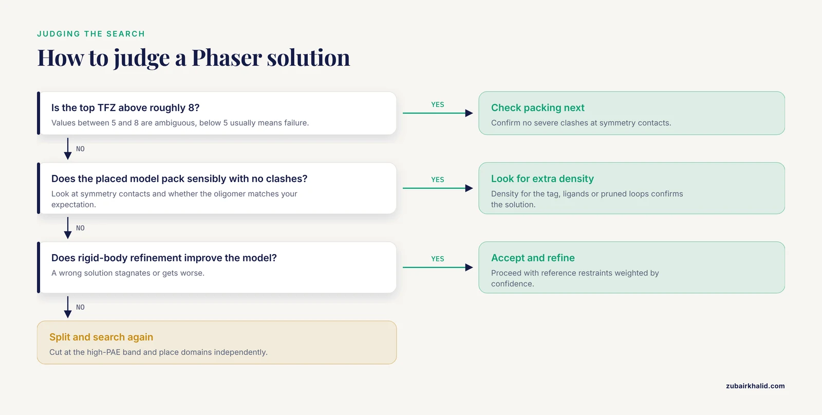
A score in the ambiguous range is not a failure and not a success. Resolve it with independent evidence:
- Run rigid-body refinement of the placed model. A correct solution improves noticeably; a wrong one stagnates or worsens.
- Compute a map and look for density corresponding to regions absent from the search model, such as your expression tag, ligands, or pruned loops. Genuine density where the model has no atoms is among the strongest available confirmations.
- Check whether the placed copy makes sensible oligomeric contacts consistent with your expectation for the protein.
Symptom: correct placement but the map is unusable in specific regions
This is usually not an MR failure but a model-bias problem in the low-confidence regions, which inherited the prediction's errors and now dominate the map. The remedy is confidence-weighted rebuilding: rebuild the low-pLDDT regions first against the map, keep the high-pLDDT regions fixed, and use the confidence scores to decide where restraints should be loose [1]. If a whole domain sits correctly but its internal detail is wrong, tighten your view to that domain and rebuild locally rather than fighting the global solution.
Symptom: the search succeeds but refinement stalls at a poor R-free
Stalling refinement after an AlphaFold-based MR solution usually means the model is over-restrained to the prediction. Relax the reference-model restraint, or restrict it to the high-confidence regions only, and let the low-confidence regions move freely against the data. The prediction should guide refinement, not imprison it.
Manual and Scripted Alternatives to the Automated Preparation Tool
phenix.process_predicted_model covers the standard cases, but three situations reward manual control: nonstandard domain definitions, cases where you want to combine residues from different confidence bands within one search model, and cases where you want to edit a multimer prediction chain by chain.
Selecting by confidence in a molecular graphics program
Both ChimeraX and PyMOL can select residues by B-factor value. In PyMOL, for example, a selection expression that keeps atoms above a chosen B-factor value lets you create a pruned object interactively, inspect exactly what is being removed, and export it. The interactive route is slower than the command-line tool but uniquely useful for one purpose: seeing what the threshold cut looks like in three dimensions before you commit to it. Watching a 100-residue tail vanish under a threshold change tells you more about whether the cut is sensible than any log file.
Scripted splitting from the raw PAE values
The PAE matrix travels as machine-readable values, typically JSON. A short script that reads the matrix, applies your chosen cutoff, and writes residue lists per domain gives you full control over boundaries. This is the right approach when the automated splitter places a boundary a few residues away from where a structural annotation says the domain edge should be, and you want to shift the boundary by hand. Keep the automated result as a reference, compare your manual boundary against it, and prefer the automated result unless you have a specific structural reason to override it.
What not to do by hand
Manual editing in a graphics program, deleting residues one by one with a mouse, is the least reproducible path and offers no advantage over scripted selection for anything but tiny one-off fixes. If you do edit by hand, save the edited file under a new name immediately and note the edit in your log, so the original prediction remains untouched as the single source of truth.
Common Misconceptions About AlphaFold Models in Crystallography
Several persistent misunderstandings cost projects time. Each one is stated here the way it usually appears in conversation, followed by the correction.
"The prediction is basically the structure, so I can skip pruning." The folded cores usually are close to the experimental structure, but the same file contains disordered tails and uncertain linkers at low confidence, and those regions are pure noise in an MR search. Pruning is not optional bookkeeping; it is the step that makes the search work.
"High pLDDT means the whole model is correct." pLDDT is a per-residue, local score. It says nothing about whether two well-scored regions are correctly positioned relative to each other. Only the PAE matrix speaks to relative orientation, and treating high local confidence as global correctness produces confident, wrong rigid bodies [1].
"The B-factors in the prediction tell me about flexibility in the crystal." They record prediction confidence, not atomic displacement. A rigid, fully ordered region of the protein that the network found hard to predict will carry a low score, and a floppy region that is trivially predictable can score high. Flexibility information comes from your experimental map and refinement, never from pLDDT.
"Side chains from AlphaFold are accurate, so I can place ligands by them." Side chains in high-confidence regions are often well placed, but binding sites are frequently exactly where the prediction and the crystal disagree, because ligand binding pulls conformations away from the free-protein ensemble the network learned. Place ligands from the experimental map, and treat predicted side-chain conformations at functional sites as suggestions to verify.
"If the model is good enough, MR is guaranteed to work." Success depends on the model, the data, and the search configuration together. Data quality, space group correctness, copy number, and resolution all bound what any search model can achieve. A strong model cannot rescue a misindexed dataset.
"Once MR succeeds, the prediction has done its job and should be discarded." The prediction remains valuable through refinement as a reference restraint, and through rebuilding as a confidence map telling you where to spend effort. Discarding it early throws away information that the experimental data alone recover only slowly [1].
"A wrong solution with a decent score will be caught later." Sometimes, but a confidently wrong MR solution can bias refinement into a self-consistent wrong model that wastes weeks. The moment to demand independent evidence is immediately after the search, not after refinement converges.
After the Solution: Carrying Confidence Information Through Refinement and Rebuilding
The preparation mindset does not end when Phaser returns a solution. The confidence metrics continue to pay off through the back end of the structure determination, and using them well shortens the path to a depositable model.
Reference restraints with a sense of proportion
Attaching the full prediction as an external reference restraint holds well-predicted regions near their correct geometry while refinement proceeds. The critical discipline is proportionality: the restraint should be strong where the prediction was confident and weak or absent where it was not. A uniform restraint applied everywhere locks in exactly the domain-orientation and loop errors that MR could not detect, converting the prediction's weaknesses into your structure's errors [1].
Prioritizing rebuilding effort
Every experienced crystallographer rebuilds under time pressure, and the confidence scores give you an objective priority order. Residues where the prediction was confident and the map agrees can be left alone. Residues where the prediction was confident and the map disagrees deserve scrutiny, because that disagreement is informative about ligand binding, crystal contacts, or conformational change. Residues where the prediction was uncertain should be rebuilt from the map with minimal regard for the prediction at all. ISOLDE, the interactive rebuilding tool in ChimeraX, uses these same confidence metrics to weight its torsion and distance restraints, which lets you pull the model toward the placed fragments and substantially reduces manual rebuilding of connecting regions [1].
When to detach the restraint entirely
As refinement progresses and the model fits the data, the prediction's influence should fade. A practical rule of thumb is to weaken or remove reference restraints once the model has been rebuilt against the map and the refinement statistics have stabilized, because at that point the experimental data are the better guide, and the restraint has already delivered its main benefit of stabilizing the early, fragile cycles.
Reproducibility: Recording the Pipeline So It Can Be Repeated
Preparation for MR involves enough small decisions that, without deliberate recordkeeping, the exact provenance of a search model becomes unrecoverable within weeks. A reproducible pipeline costs little and pays off during manuscript preparation, deposition, and any future reprocessing.
Directory and naming conventions
A workable layout separates immutable inputs from generated intermediates:
project/
  data/data.mtz
  construct/construct.fasta
  prediction/ranked_0.pdb
  prediction/pae.json
  prepared/t70_pa8_full.pdb
  prepared/t70_pa8_d1.pdb
  prepared/t70_pa8_d2.pdb
  mr/full_t70.log
  mr/domains_t70.log
  refine/...
The prepared file names encode the threshold and cutoff used, so any file on disk announces its own provenance. The prediction directory is never modified after download.
What to log
For each MR attempt, record the search model file, the Phaser command or GUI settings, the top TFZ and LLG, and a one-line interpretation. For each preparation run, record the tool version, the full parameter set, and the reported segment boundaries. Version numbers matter because tool behavior and defaults can shift between releases; the habit of running commands with a flag that lists current defaults, mentioned earlier in this guide, is also your record of what a given version actually did.
Scripts over clicks
GUI workflows are fine for exploration, but the pipeline you intend to reproduce should exist as a small shell script or notebook that runs from raw inputs to the final refined model. When a reviewer, a collaborator, or your future self asks how the search model was made, the answer should be a file, not a reconstruction from memory.
When Molecular Replacement Is the Wrong First Move
AlphaFold models are so effective that MR has become the default first attempt for almost everything, and that is mostly healthy. But two situations deserve a deliberate pause before committing to it.
Cases where the prediction misleads systematically
Proteins whose crystal conformation depends strongly on ligand binding, large conformational states, or cofactor-induced rearrangements can adopt a substantially different arrangement in the crystal than in the prediction. If you know from biochemistry that your protein undergoes a large ligand-dependent motion, expect the prediction to represent the unbound state, plan for domain splitting from the start, and treat a failed full-length search as expected rather than alarming.
Cases where experimental phasing is the better investment
If your construct contains selenomethionine labeling, an inherent heavy atom, or a bound metal giving an anomalous signal, experimental phasing provides unbiased phases that no model can match, and it simultaneously validates the MR result if you pursue both. When a project has already consumed days on failed MR, adding an experimental phasing route is usually faster than a fourth round of model surgery. And when trimming, splitting, and hybrid approaches have all been exhausted, the documented direct-methods hybrid framework offers a distinct, model-error-tolerant path that is worth attempting before concluding the structure is unsolvable [2].
The judgment call underlying all of these sections is the same one underlying the whole guide: the AlphaFold model is an extraordinarily good hypothesis about your molecule, complete with a quantified statement of where the hypothesis is shaky. Molecular replacement succeeds with these models when you read that statement carefully, act on it during preparation, and keep treating the experimental map, never the prediction, as the final authority.
Frequently Asked Questions
What pLDDT cutoff should I use when preparing an AlphaFold model for molecular replacement?
Start with 70, which is the default in phenix.process_predicted_model and works for most targets [1]. If MR fails with a well-behaved dataset, raise the cutoff toward 85 to make a cleaner, more conservative model, and try a lower cutoff near 60 only if you suspect the low-confidence region is actually ordered in your crystal.
Should I submit the full-length AlphaFold model or split it into domains?
Split it when the PAE matrix shows confidently predicted blocks separated by bands of high inter-domain PAE, and use it whole when the matrix is uniformly low [1]. When in doubt, run both and compare the TFZ scores.
Can I use a model from the AlphaFold server or the AlphaFold Protein Structure Database directly, or do I need a new prediction?
You can use database models directly after downloading, since they include the pLDDT values and PAE matrix that the preparation tools need. Only run a new prediction, through the AlphaFold server or ColabFold, if the database lacks your sequence, you need a multimer prediction, or your construct differs substantially from the database entry.
Do I need to remove side chains or trim low-confidence loops before running Phaser?
Pruning low-confidence residues is usually sufficient, and leaving well-predicted side chains in place adds useful scattering signal. Stripping side chains is an older homology-modeling habit that generally hurts more than it helps with AlphaFold-quality models.
How do I know whether my molecular replacement solution is correct?
Look for a TFZ score above roughly 8, a large LLG gain, sensible packing with no clashes at symmetry contacts, and a map that shows clear density for regions absent from the search model. A single borderline score without supporting evidence should be treated as unverified.
What if the AlphaFold model has the wrong domain orientation relative to my crystal?
Split the model at the high-PAE boundary and search the domains independently, then let refinement and rebuilding find the correct inter-domain geometry. If that also fails, hybrid strategies combining molecular replacement with direct-methods dual-space iteration are designed to correct exactly this kind of phase error and model bias from a full-length starting model [2].
Can AlphaFold models be used for multimeric targets and complexes?
Yes. Predicted complexes from the AlphaFold server or AlphaFold-Multimer can serve as MR search models, and predicted complex models are among the use cases highlighted for confidence-guided preparation [1]. Confirm that the predicted stoichiometry and interface match the content of your asymmetric unit before searching.
How accurate does an AlphaFold model need to be for molecular replacement to succeed?
No fixed accuracy threshold exists, because success depends on model size, data quality, and resolution together. What the published test cases show is that models whose folded cores are accurate, with local errors and domain orientation errors handled by pruning, splitting, and confidence-weighted refinement, solve structures that homology models at low sequence identity could not [1].