AlphaFold Local Installation Requirements
By Dr. Zubair Khalid, DVM, MS, PhD ·
By the end of this article you will be able to judge whether your workstation or lab server can run AlphaFold locally, install AlphaFold2 or AlphaFold3 end to end, prepare an input file in the correct format, run your first prediction, and read the confidence scores in the output. The walkthrough doubles as an alphafold tutorial for a first monomer structure, and the later sections cover the input formats, template handling, and the hosted alternatives that remove the need for a local install altogether.
Before you start, you should have on hand:
- A Linux machine (Ubuntu 22.04 or similar) with an NVIDIA GPU of at least 16 GB memory
- Sudo rights on that machine
- Roughly 560 GB to 2.6 TB of free disk space for the genetic databases, depending on the preset you choose
- A protein sequence in FASTA format
- Docker or Apptainer installed, or the willingness to install one of them
If your hardware does not meet these numbers, skip to the section on hosted options. ColabFold-based workflows have been used successfully in published work precisely because they require no local installation or computation [1].
What "Local Installation" Actually Means
AlphaFold is not a single program. A local installation bundles four things: the model code and trained network weights, a numerical computing stack built on JAX, a container runtime so the software dependencies stay reproducible, and a set of large reference databases used to build the multiple sequence alignment (MSA, a column-wise alignment of your protein against sequences from related organisms) and to search for structural templates.
A common source of confusion is that different versions of AlphaFold have different needs. AlphaFold2, released in 2021, runs monomers and complexes and is the version most lab clusters still use. AlphaFold3, released in 2024, adds ligands, nucleic acids, and chemically modified residues, and it uses a different input format and a different set of databases. The alphafold local installation requirements for each are summarized below.
AlphaFold Local Installation Requirements at a Glance
The numbers in this table come from the official AlphaFold2 and AlphaFold3 repository documentation maintained by Google DeepMind. Treat them as the documented baseline rather than generous estimates.
| Requirement | AlphaFold2 (minimum practical) | AlphaFold2 (recommended) | AlphaFold3 (documented recommendation) |
|---|---|---|---|
| Operating system | Linux | Linux | Linux |
| GPU memory | 16 GB (works for monomer) | 40 GB NVIDIA A100 | 40 GB NVIDIA A100 |
| Host RAM | 32 GB | 64 GB | 64 GB |
| Disk for databases | About 560 GB (reduced preset) | About 2.6 TB (full preset) | About 2 TB |
| Container runtime | Docker or Apptainer | Docker or Apptainer | Docker |
| Disk for container and weights | Under 50 GB | Under 50 GB | About 100 GB |
Two notes on this table. First, CPU-only inference is technically possible with AlphaFold2 through a -use_gpu_relax false configuration, but a single prediction can take many hours to days, so most groups treat a GPU as mandatory. Second, the database disk figure is the dominant cost. The full preset includes the BFD database of about 2.2 billion protein sequences, and the reduced preset swaps BFD for the smaller Small BFD to cut the download by roughly a factor of five at a modest cost in prediction quality for hard targets.
Hardware Requirements in Detail
GPU
JAX, the library AlphaFold is built on, uses the XLA compiler to target NVIDIA GPUs. For AlphaFold2 monomer prediction, any NVIDIA card with 16 GB of memory will run the default five model evaluations, though the relaxation stage and multimer runs are the usual points of failure on smaller cards. For AlphaFold3, the official documentation recommends a single A100 40 GB and states that smaller 16 GB cards can work for shorter inputs with adjusted settings.
You can check what your machine has with:
nvidia-smiExpected output looks like this (abbreviated):
+-----------------------------------------------------------------------------+
| NVIDIA-SMI 535.129.03   Driver Version: 535.129.03   CUDA Version: 12.2     |
|-------------------------------+----------------------+----------------------+
| GPU  Name        Persistence-M| Bus-Id        Disp.A | Volatile Uncorr. ECC |
|   0  NVIDIA A100-SXM4      On | 00000000:07:00.0 Off |                    0 |
|  40C    P0              45W / 400W |      0MiB /  40960MiB |      0%      Default |
+-----------------------------------------------------------------------------+
If nvidia-smi is not found, install the NVIDIA driver before anything else. The driver version must support the CUDA runtime shipped inside the AlphaFold container, so install the newest vendor driver your cluster permits rather than a distribution-packaged one.
RAM and disk
Host RAM matters during MSA generation and feature construction. Sequence databases such as UniRef90 and MGnify are loaded into memory during preprocessing, and 64 GB keeps the full pipeline comfortable. Disk needs are dominated by the genetic databases plus working space for MSA outputs, which grow quickly when you predict many sequences in batch.
Software Stack Requirements
- Linux with the NVIDIA driver. The official pipelines target Linux. Windows users should install WSL2 with CUDA passthrough or run on a remote Linux server.
- Docker with the NVIDIA Container Toolkit so containers can access the GPU, or Apptainer (formerly Singularity) on shared HPC systems where Docker is not permitted.
- Python 3 on the host, mainly to drive the download and run scripts. The heavy Python dependencies (JAX, Haiku, TensorFlow for AlphaFold2, JAX and hmmpytm for AlphaFold3) live inside the container, which is the point of the container approach.
- The model weights. AlphaFold2 weights are openly downloadable via the repository scripts. AlphaFold3 weights are provided for free under terms of use that restrict commercial applications, and you must request access and agree to those terms before downloading them.
A quick preflight check that catches most early failures:
nvidia-smi
docker --version
docker run --rm --gpus all nvidia/cuda:12.2.2-base-ubuntu22.04 nvidia-smi
free -g
df -h /path/to/your/databases
The third command is the decisive one. If the GPU table prints from inside the container, the container toolkit is wired up correctly and AlphaFold will see your card.
Genetic Databases and How to Download Them
AlphaFold2 needs seven database sets: UniRef90, UniProt (clusters), UniRef100, MGnify, PDB70 or the mmCIF structures for templates, BFD (or Small BFD), and PDB seqres. The repository ships scripts that download and unpack all of them.
git clone https://github.com/google-deepmind/alphafold.git
cd alphafold

# Full preset, about 2.6 TB
./scripts/download_all_data.sh /data/alphafold/databases

# Reduced preset, about 560 GB, omits BFD in favor of Small BFD
./scripts/download_all_data.sh /data/alphafold/databases reduced_dbs
Expected output during a healthy download looks like:
Downloading UniRef90 v2021.03...
Finished downloading UniRef90 v2021.03.
Downloading MGNIFY v2021.09...
The script verifies and unpacks each archive. If a download is interrupted, rerun the same command, because completed archives are skipped. Plan the download over several days on a typical institutional connection, and run it inside tmux or screen so a dropped SSH session does not kill it.
AlphaFold3 uses a different, smaller set of public databases for its JackHMMER-based MSA search, downloaded by scripts in the AlphaFold3 repository, plus the model parameter package you obtain after accepting the terms of use.
Step-by-Step Walkthrough: Your First AlphaFold2 Prediction
This is the alphafold local installation requirements example most people need first: one protein chain, one GPU, one output directory.
1. Prepare the input FASTA
>LYSC_CHICK|Hen egg white lysozyme
KVFGRCELAAAMKRHGLDNYRGYSLGNWVCAAKFESNFNTQATNRNTDGSTDYGILQINSRWWCNDGRTPGSRNLCNIPCSALLSSDITASVNCAKKIVSDGNGMNAWVAWRNRCKGTDVQAWIRGCRL
Chain identifiers use UniProt conventions in AF2, and for multimer jobs each FASTA entry becomes one chain with a unique name.
2. Build the container
cd alphafold
docker build -f docker/Dockerfile -t alphafold .
3. Run the prediction
The repository provides a run script that assembles the full Docker command and resolves individual database paths from your data directory:
python3 scripts/run_alphafold.py \
  --fasta_paths=/data/inputs/lysozyme.fasta \
  --output_dir=/data/outputs \
  --data_dir=/data/alphafold/databases \
  --db_preset=full_dbs \
  --model_preset=monomer \
  --max_template_date=2021-11-01 \
  --use_gpu_relax=true
Key parameters explained:
| Parameter | What it controls | When to change it |
|---|---|---|
-db_preset | Full versus reduced genetic databases | Use reduced_dbs if you downloaded the smaller preset |
-model_preset | monomer, monomer_casp14, or multimer | Use multimer for complexes with more than one chain |
-max_template_date | Cutoff for structural templates used | Set earlier than your benchmark release date to prevent template leakage in method evaluation |
-num_multimer_predictions | Number of multimer model runs (default 5) | Raise for better complex ranking if GPU memory and time allow |
-use_gpu_relax | Run the Amber relaxation on GPU | Set to false only on CPU-only runs |
On a 40 GB A100, a 130-residue monomer with a good MSA finishes all five models in roughly 20 to 40 minutes. On a 16 GB card, expect the same job to take closer to an hour.
4. Inspect the output
outputs/lysozyme/
├── ranked_0.pdb
├── ranked_1.pdb
├── ranked_2.pdb
├── ranked_3.pdb
├── ranked_4.pdb
├── scores_ranked_0.json
├── pae_ranked_0.png
├── plddt_ranked_0.png
├── msas/
└── timings.json
ranked_0.pdb is the best-scoring model. The per-residue confidence (pLDDT) is stored in the B-factor column of the PDB file, and scores_ranked_0.json contains the full predicted aligned error (PAE) matrix and interface metrics for complexes. Open the PDB in PyMOL or ChimeraX and color by B-factor to see the confidence gradient on the structure.
5. Verify the result is credible
Check three things before you trust a model. First, mean pLDDT: values above 90 indicate very high backbone accuracy, 70 to 90 confident, 50 to 70 low, and below 50 typically disordered. Second, the PAE matrix: strong interfaces between chains should show low (dark) PAE across the inter-chain blocks. Third, for complexes, the ipTM score in the ranking: predictions with low ipTM are often wrong relative to the true binding mode even when each chain individually looks excellent.
One refinement on scoring comes from method evaluation work. In a benchmark of short linear motif (SLiM) interactions, a compact interaction module embedded in disordered protein regions, the MiniPAE metric was identified as the most suited AlphaFold metric for screening SLiM-mediated interactions, outperforming raw interface confidence reads for that use case [1]. If your question is whether a short peptide binds a folded domain, look at MiniPAE rather than global pLDDT.
AlphaFold Local Installation Requirements Format: Input Files Explained
The word "format" in this context covers three distinct layers: the sequence input, the MSA input, and, for AlphaFold3, a structured job specification.
FASTA for AlphaFold2
A multimer job with two chains is a single FASTA file with two entries:
>chainA|UniProt description here
MKTAYIAKQRQISFVKSHFSRQ...
>chainB|second protein
GGGTYSGPRTGKYKPTG...
Every chain name must be unique. Non-standard residues in the sequence are rejected, so strip them or let the pipeline's preprocessing handle known mappings.
JSON for AlphaFold3
AlphaFold3 replaces FASTA with a JSON job specification that can encode proteins, nucleic acids, ligands, ions, and modifications in one file:
{
  "name": "lysozyme_monomer",
  "modelSeeds": [1],
  "sequences": [
    {
      "protein": {
        "id": "A",
        "sequence": "KVFGRCELAAAMKRHGLDNYRGYSLGNWVCAAKFESNFNTQATNRNTDGSTDYGILQINSRWWCNDGRTPGSRNLCNIPCSALLSSDITASVNCAKKIVSDGNGMNAWVAWRNRCKGTDVQAWIRGCRL"
      }
    }
  ],
  "dialect": "alphafold3",
  "version": 2
}
The run command mirrors AF2 in shape:
python run_alphafold.py \
  --json_path=lysozyme_monomer.json \
  --model_dir=/data/af3/params \
  --output_dir=/data/outputs
Providing your own MSA
If you already have an A3M or Stockholm alignment from your own search, both AF2 and AF3 accept it, which cuts runtime to minutes because the slow database scans are skipped. This is standard practice for large batch jobs.
Template Requirements: Using Structural Templates
Templates are experimentally solved structures (from the PDB, the global repository of macromolecular structures maintained by the worldwide Protein Data Bank partnership) that AlphaFold aligns to your target as additional geometric information. Three requirements matter locally.
- The mmCIF template database. AlphaFold2 downloads PDB mmCIF files as part of its data setup, and template search runs against them during preprocessing.
-max_template_date. This flag controls how recent a template may be. For benchmarking a prediction method, set it before the evaluation targets were published, otherwise the model can effectively look up the answer. For routine use, the default behavior of using all available templates is fine.- Custom templates. When your target is related to an in-house structure not yet in the PDB, both AlphaFold3's pipeline and wrapper tools support supplying custom template files directly. ABCFold, for example, provides straightforward options to use templates, including custom templates, as part of its standardized input [2].
A common mistake is assuming templates are required for good accuracy. For most folded proteins the MSA carries most of the signal, and templates mainly help for fast-evolving or MSA-poor families.
Avoiding the Database Download Entirely: The MMseqs2 Route
The single largest barrier in the alphafold local installation requirements is disk. There is a documented way around it. ABCFold, a Python and JavaScript wrapper for running and comparing AlphaFold 3, Boltz-1, and Chai-1, can generate MSAs internally with either the JackHMMER search bundled with AlphaFold 3 or with the MMseqs2 API, and this allows AlphaFold 3 to be installed and run without downloading the large databases needed for JackHMMER [2]. The tradeoff is that MSA quality now depends on a remote web service, so results can shift if the API changes or is down, and very large screening jobs become network-bound.
The practical decision rule: download the full databases if you will run hundreds of predictions or need reproducibility against a frozen database version, use the MMseqs2 API route if you need to get started today on a machine with limited disk.
Hosted Alternatives: When Local Installation Is Not the Right Choice
If you lack a GPU, two hosted paths cover most needs.
AlphaFold Server. Google DeepMind operates a free web server for AlphaFold3 for non-commercial use. You paste or upload sequences for proteins, nucleic acids, and ligands, and the server returns structures and confidence metrics. There are limits on job volume and input size, and the terms of use restrict commercial applications, so check both before relying on it for a project.
ColabFold notebooks and local ColabFold. ColabFold packages AlphaFold2 with the MMseqs2 API for MSA generation and runs in a browser notebook, requiring no local installation or computation. Published method-evaluation work on SLiM discovery used AlphaFold via ColabFold as a practical and accessible route, and the same study provides a streamlined and cost-effective AlphaFold analysis workflow requiring no local installation for screening short linear motifs [1]. For batch work, ColabFold also installs locally with far lighter requirements than stock AlphaFold2, because MMseqs2 replaces the JackHMMER database stack:
conda create -n colabfold python=3.11
conda activate colabfold
pip install "colabfold[alphafold-minus-jax]"
colabfold_batch --msa-mode mmseqs2_uniref_env --num-models 5 lysozyme.fasta results/
This is often the fastest route from a sequence to a structure on a modest workstation, at the cost of depending on a public MSA service.
Running AlphaFold 3 Alongside Boltz-1 and Chai-1 with ABCFold
Once you have a working AF3 setup, a wrapper can simplify daily use. ABCFold was built because preparing inputs for locally installed structure prediction software is not always straightforward and results are not always presented in an accessible fashion. It takes a standardized input, installs Boltz-1 and Chai-1 at runtime if needed, and treats results from all packages in a unified fashion so predictions from different methods can be compared directly, with visualization options that include information on steric clashes [2]. All scripts and documentation are available on GitHub and PyPI, and installation follows the usual Python pattern:
pip install ABCFoldFor labs evaluating whether AlphaFold3's ligand and nucleic acid handling is the right fit for a given complex, the ability to run the same standardized input through AF3, Boltz-1, and Chai-1 and compare outputs side by side is the main reason to set ABCFold up after your base installation works.
Common Mistakes and Limitations
- Underestimating disk. People download the full 2.6 TB preset onto a 1 TB volume and fill the disk at hour nine of the download. Check
df -hbefore starting and prefer the reduced preset unless you specifically need BFD. - Driver and CUDA mismatches. The error
nvidia-container-cli: requirement error: unsatisfied condition: cuda=X.Ymeans your host driver is too old for the container. Upgrade the driver, not the container. - Docker on shared HPC systems. Many clusters forbid Docker daemons. Use Apptainer to pull and convert the AlphaFold image, or run through your cluster's container module.
- Template leakage during benchmarking. Leaving
-max_template_dateat its default while evaluating a method on published structures means templates of your test cases can enter the model. Always pin the date for evaluation work. - Out-of-memory on multimer jobs. The message
CUDA_ERROR_OUT_OF_MEMORYon a 16 GB card during multimer means the model run plus relaxation exceeded memory. Reduce-num_multimer_predictions, shorten the chains, or move to a 40 GB card. - Confusing interface confidence with per-chain confidence. A complex can rank well on per-chain pLDDT while the relative positioning of the chains is wrong. Read the PAE matrix and ipTM, and for short peptide questions such as SLiM binding, use a metric designed for that scale such as MiniPAE [1].
- Over-reading predictions for degenerate, transient interactions. A blind-screening evaluation of SLiM-like interactions, built as an unbalanced dataset with a large excess of non-binders to mimic real-world screening, revealed a critical limitation in AlphaFold's specificity for SLiM detection, and the authors proposed an adaptive scoring threshold to compensate [1]. Treat negative screening results with skepticism and validate candidates experimentally.
- Reproducibility drift. Database versions and the MMseqs2 API content change over time. Record your
-db_preset, database versions, model version, and-max_template_datewith every result.
Choosing an Installation Route: A Decision Comparison
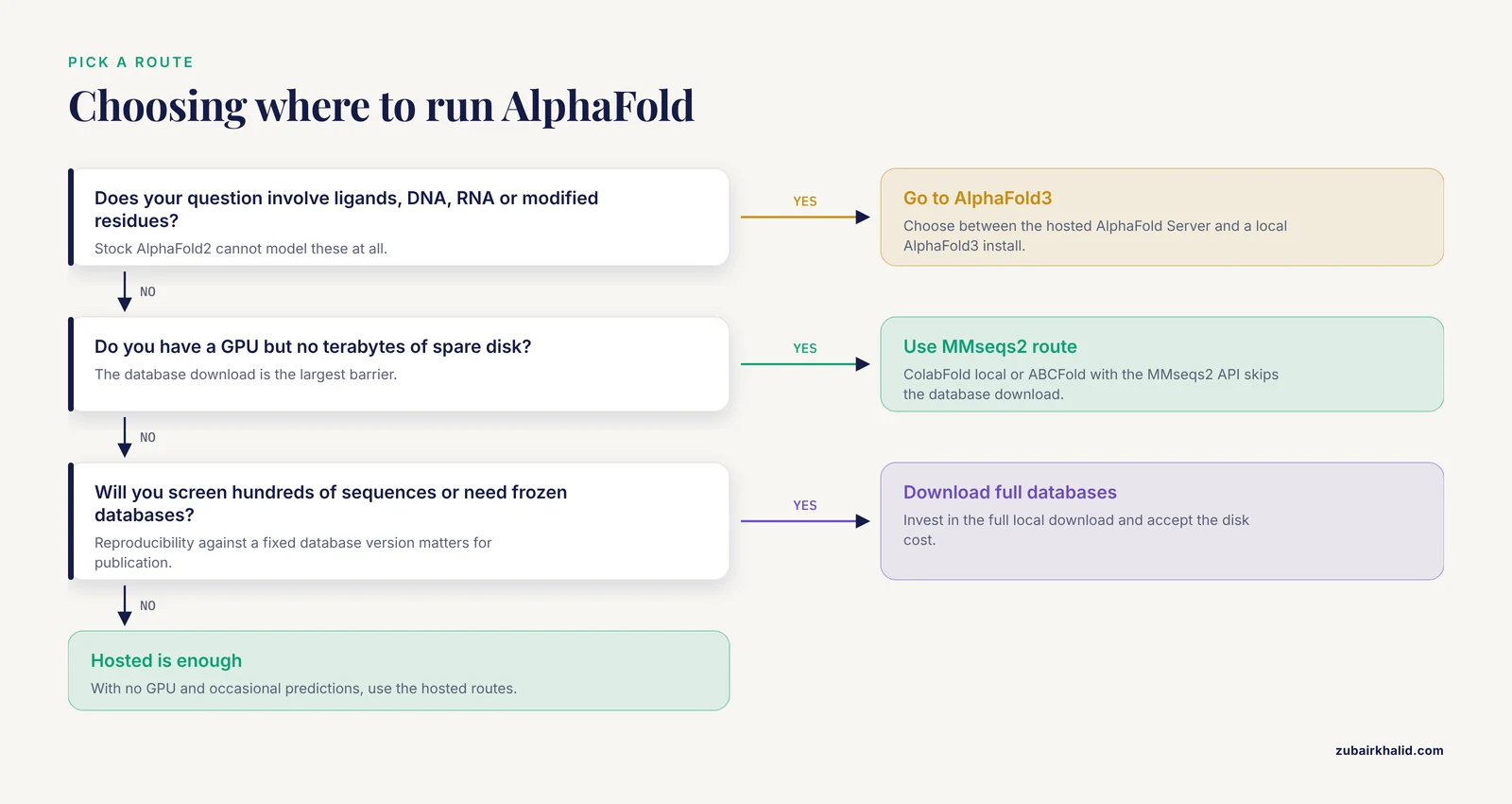
Before touching a terminal, decide which of the four installation routes fits your situation. Choosing wrong at this stage is the most expensive mistake in this whole process, because the database download alone can consume days of bandwidth and most of a storage volume.
The four routes differ along five axes: disk footprint, runtime per prediction, control over inputs, suitability for batch work, and licensing constraints.
| Route | Disk needed | Best for | Main limitation |
|---|---|---|---|
| - | - | - | - |
| Stock AlphaFold2 (Docker or Apptainer) | About 560 GB to 2.6 TB for databases | Reproducible batch monomer and multimer work on your own hardware | Large download, Docker often blocked on shared clusters |
| ColabFold local | Far less than stock AF2, because MMseqs2 replaces the local JackHMMER stack | Fast single predictions on a modest workstation | Depends on a public MSA API, lighter reproducibility guarantees |
| AlphaFold3 local | About 2 TB for databases and parameters | Complexes with ligands, nucleic acids, and modified residues | Weight access requires agreeing to terms that restrict commercial use |
| AlphaFold Server (hosted) | None | Non-commercial AF3 predictions with no hardware at all | Job volume and input size limits, commercial use restricted |
A practical decision sequence looks like this. First, if your question involves small molecules, DNA or RNA, or chemically modified residues, stock AlphaFold2 cannot help you at all, so your real choice is between the AlphaFold Server and a local AlphaFold3 install. Second, if you have a GPU but no terabytes of spare disk, ColabFold local or the ABCFold wrapper with the MMseqs2 API route gets you running without the database download, since ABCFold can generate MSAs through the MMseqs2 API and thereby allow AlphaFold 3 to run without the large JackHMMER databases [2]. Third, if you plan to screen hundreds of sequences, or you need results frozen against a specific database version for a publication, invest in the full local database download and accept the disk cost. Fourth, if you have no GPU at all and only occasional predictions to run, the hosted routes are the correct answer, and ColabFold notebooks have been used in published evaluation work precisely because they require no local installation or computation [1].
One more consideration that people often discover too late: reproducibility. Any route that depends on a remote MSA service inherits that service's database state at query time. If a reviewer asks you to rerun a prediction eighteen months later and get the identical alignment, a locally frozen database snapshot makes that trivial and a remote API makes it impossible to guarantee. Labs that treat structure prediction as part of a reproducible pipeline almost always end up maintaining local databases, which is why the full-download route remains the backbone of serious local usage despite its cost.
Preparing the Host Machine: A Full Setup Walkthrough
The article so far assumes a machine that already has its driver and container runtime sorted out. Most failed first installations fail at exactly this stage, so here is the full host preparation sequence for a fresh Ubuntu 22.04 machine, step by step, with the checks that confirm each layer before you move to the next.
Step 1: Install the NVIDIA driver
The container carries its own CUDA runtime, so what the host needs is only the kernel driver, and it needs to be recent enough for the CUDA version inside the container. The cleanest path on Ubuntu is to add the graphics drivers repository and install the vendor metapackage:
sudo apt update
sudo apt install ubuntu-drivers-common
ubuntu-drivers devices          # lists recommended driver
sudo apt install nvidia-driver-535   # or the version your cluster mandates
sudo reboot
After reboot, verify:
nvidia-smiIf this prints a GPU table, the driver layer is done. If it prints nothing or complains about a missing device, the most common causes are a secure boot setting that blocks the unsigned module, or a leftover distribution driver conflicting with the one you just installed. Resolve this before proceeding, because every later failure will be harder to diagnose with a broken driver underneath.
Step 2: Install Docker and the NVIDIA Container Toolkit
Docker itself is straightforward, but the piece people forget is the NVIDIA Container Toolkit, which is what lets a container see the GPU:
sudo apt install docker.io
sudo systemctl enable -now docker
Then install the NVIDIA Container Toolkit per NVIDIA's current repository instructions, which typically reduce to adding the toolkit repository and running:
sudo apt install nvidia-container-toolkit
sudo nvidia-ctl configure -runtime=docker  # example; follow the toolkit's own docs for your version
sudo systemctl restart docker
The verification command is the decisive one from the preflight check in the main article:
docker run -rm -gpus all nvidia/cuda:12.2.2-base-ubuntu22.04 nvidia-smiIf the GPU table prints from inside the container, stop configuring and move on. If you see docker: permission denied, your user is not in the docker group; either run with sudo or add yourself with sudo usermod -aG docker $USER and log out and back in. If you see nvidia-container-cli: requirement error: unsatisfied condition: cuda=X.Y, the host driver is too old for the CUDA version the container requests, and the fix is a driver upgrade on the host, not a different container.
Step 3: The Apptainer alternative for shared systems
On university clusters, the Docker daemon is frequently forbidden for security reasons, and Apptainer is the sanctioned alternative. Apptainer can convert the standard AlphaFold Docker image without a daemon:
apptainer pull alphafold.sif docker://alphafold-image-referenceTwo behavioral differences matter once you switch. First, Apptainer runs containers with your user identity by default rather than root, which means output directories must be writable by you, which is usually what you wanted anyway. Second, GPU access is requested with the -nv flag rather than -gpus all, and a missing -nv flag produces a container that runs but silently falls back to CPU, which manifests as predictions that are inexplicably slow rather than errors. That silent failure mode is worth memorizing, because it wastes hours of cluster time before anyone notices.
Step 4: Create the directory skeleton
Establish the layout before anything large arrives, because renaming a 2.6 TB directory after the fact is painful:
sudo mkdir -p /data/alphafold/{databases,containers,inputs,outputs,logs}
sudo chown -R $USER /data/alphafold
Points to check before the download: confirm the target filesystem has space with df -h /data/alphafold/databases, confirm it is not an NFS mount with tight quotas if you expect terabyte-scale writes, and confirm the filesystem supports the number of small files the unpacked databases will produce. Some institutional scratch filesystems enforce per-directory file limits that archive unpacking can hit.
Running AlphaFold on an HPC Cluster with SLURM
Many readers will not own the GPU at all; they will share an A100 through a scheduler. The workflow differs from a workstation in three ways: the container runtime is usually Apptainer, databases usually live on a shared read-only path maintained by the HPC staff, and each prediction becomes a batch job.
A minimal SLURM submission script for a monomer prediction looks like this:
#!/bin/bash
#SBATCH -job-name=af2_lysozyme
#SBATCH -gres=gpu:1
#SBATCH -cpus-per-task=8
#SBATCH -mem=64G
#SBATCH -time=04:00:00
#SBATCH -o af2_%j.log

module load apptainer
module load cuda

apptainer exec -nv \
  -bind /shared/alphafold/databases:/data/databases:ro \
  -bind /scratch/$USER/outputs:/data/outputs \
  /shared/alphafold/containers/alphafold.sif \
  python /app/alphafold/run_alphafold.py \
    -fasta_paths=/data/outputs/lysozyme.fasta \
    -output_dir=/data/outputs \
    -data_dir=/data/databases \
    -db_preset=full_dbs \
    -model_preset=monomer \
    -max_template_date=2021-11-01 \
    -use_gpu_relax=true
Submit it with sbatch af2_lysozyme.sh and monitor with squeue -u $USER. Several cluster-specific notes deserve attention.
First, CPU allocation matters as much as GPU allocation during preprocessing. JackHMMER and the template search are CPU-bound and parallelized across threads, so an under-provisioned -cpus-per-task value turns the MSA stage into the bottleneck even on a fast GPU. The article's timing estimate of roughly 20 to 40 minutes for a 130-residue monomer on a 40 GB A100 assumes the CPU side is not starving the GPU; on a badly configured cluster job the same prediction can take several hours with the GPU idle most of the time.
Second, check whether your cluster already maintains the AlphaFold databases. Large facilities often host them at a shared path precisely because dozens of users should not each store 2.6 TB. If they do, mount that path read-only as shown above and skip the entire download section. Ask your HPC staff or check the facility's software pages before you start downloading anything.
Third, mind the scheduler's scratch policy. Many clusters purge scratch directories after a fixed retention period, and AlphaFold's msas/ output directory is exactly the kind of intermediate data you want to keep if you plan to rerun with different model settings but the same alignment. Copy MSAs to durable storage as part of your post-job step rather than assuming scratch persists.
Fourth, for repeated submissions, wrap the per-protein logic in a loop or an array job. A common pattern is a directory of FASTA files plus a submission script that iterates over them and launches one SLURM job each, so the queue parallelizes your batch instead of one job serializing it.
Building Better MSAs: Depth, Sources, and Custom Alignments
The MSA is where most prediction quality is won or lost, yet it is the part of the pipeline people understand least, partly because the default scripts make it invisible. A short primer on what happens under the hood will help you diagnose the failure mode where a prediction simply looks wrong.
What the pipeline actually does
For a protein sequence, AlphaFold2's preprocessing runs iterative searches against UniRef90, MGnify, UniProt clusters, and BFD or Small BFD using JackHMMER and HHblits, collects the hit sequences, aligns them, and produces a deep multiple sequence alignment that the network consumes alongside the raw sequence. Template search against PDB structures runs in parallel. The network never sees your databases directly; it sees only the MSA features and template features built from them.
Why MSA depth matters and when it does not
For a protein belonging to a large, well-sampled family, the search returns thousands of homologs and the co-evolutionary signal within that alignment is what lets the model infer contacts across the fold. For a protein from a small family, an orphan sequence, a rapidly evolving domain, or a designed protein, the MSA comes back shallow, and accuracy degrades. This is not a configuration error you can fix with a flag; it is a property of the sequence you submitted.
There are partial mitigations. Widening the search databases (the full preset with BFD, rather than the reduced preset) improves recovery for hard targets, which is exactly the tradeoff the reduced preset makes explicit: smaller download, modest cost in prediction quality for difficult sequences. Alternatively, if you know the protein has close homologs that the standard databases miss, for example because they are from a niche taxonomy or from patent sequence collections, you can build a custom MSA with your own search tools and supply it directly. Both AF2 and AF3 accept precomputed A3M or Stockholm alignments, and doing so cuts runtime to minutes because the slow database scans are skipped entirely.
A worked custom-MSA workflow
The practical sequence for supplying your own alignment is:
- Run your own homology search with whatever tool your lab trusts, collecting homologous sequences in unaligned FASTA form.
- Align them with a standard multiple sequence alignment tool and convert to A3M format, which is essentially aligned FASTA with lowercase letters marking insertions relative to the query.
- Ensure the first sequence in the file is your target query sequence, unmodified, because AlphaFold uses it to establish the residue indexing.
- Pass the alignment to the pipeline through its custom MSA input mechanism rather than the default search path.
One caution: a custom MSA built with different search parameters than the pipeline's defaults is a scientific choice, not just an engineering shortcut, and it should be recorded in your methods section. Reviewers increasingly ask for MSA provenance, and a result obtained from a hand-built alignment cannot be reproduced from the pipeline defaults alone.
Diagnosing a shallow MSA
The output directory's msas/ folder tells you what the search actually recovered. If your target returned only a handful of sequences and the model produces a structure with low pLDDT in the core, the likeliest explanation is not a broken installation but a genuine lack of evolutionary information. In that regime, templates carry relatively more weight, and supplying a related experimental structure as a template is one of the few levers that meaningfully helps, as covered in the template section of the main article.
A Multimer Worked Example: Predicting a Two-Chain Complex
Monomer predictions are the tutorial case; complexes are where local installations earn their keep, because hosted services constrain input size and batch throughput. Here is a complete two-chain walkthrough using the multimer preset.
The input
For a heterodimer of a folded domain and a short binding partner, the FASTA contains both entries:
>chainA|Folded domain protein
MKTAYIAKQRQISFVKSHFSRQLEWLSN...
>chainB|Binding peptide
GGGTYSGPRTGKYKPTG...
Two formatting points that cause real failures. Every chain name must be unique, and duplicates produce confusing errors downstream rather than a clean rejection. Also, chain length asymmetry is handled fine by the model, but extremely short chains relative to the partner are the classic hard case, for reasons the confidence section below makes concrete.
The run
python3 scripts/run_alphafold.py \
  -fasta_paths=/data/inputs/heterodimer.fasta \
  -output_dir=/data/outputs \
  -data_dir=/data/alphafold/databases \
  -db_preset=full_dbs \
  -model_preset=multimer \
  -num_multimer_predictions=5 \
  -max_template_date=2021-11-01 \
  -use_gpu_relax=true
The multimer preset runs each of the multimer models and ranks the resulting complexes. Because each prediction is a full model run per chain pairing, multimer jobs cost proportionally more GPU time and memory than monomer jobs, which is why 16 GB cards struggle here and why the memory table in the main article recommends 40 GB for serious work.
Reading the result
The ranking logic differs from the monomer case in one crucial way. For monomers, ranking tracks overall structure confidence. For complexes, the interface score, ipTM, dominates, because a complex model can have every residue beautifully confident in its own local fold while the two chains are docked in a relative orientation that is simply wrong. Before you report an interface, open the PAE matrix image and examine the cross-blocks: the off-diagonal blocks that represent chain A against chain B. Dark, low-error cross-blocks mean the model placed the interface consistently across the prediction; pale cross-blocks mean the relative arrangement is a guess.
For the specific and common case of a short linear motif binding a folded domain, the standard metrics behave poorly, and dedicated evaluation work has addressed this directly. In a benchmark of SLiM-mediated interactions, the MiniPAE metric was identified as the most suited AlphaFold metric for screening those interactions, outperforming raw interface confidence reads [1]. If your two-chain job is exactly this pattern, a short peptide against a domain, consult that metric rather than trusting the headline ranking.
A further caution from the same evaluation literature applies to anyone using multimer predictions for discovery rather than description: a blind-screening evaluation built as an unbalanced dataset with a large excess of non-binders, designed to mimic real-world screening conditions, revealed a critical limitation in AlphaFold's specificity for SLiM detection, and the authors proposed an adaptive scoring threshold to compensate [1]. The lesson generalizes beyond motifs: the ranking score is calibrated for typical complexes, and when your input distribution departs from typical, treat the ranking as a hypothesis generator that needs experimental follow-up.
AlphaFold3 JSON Inputs Beyond Proteins: Ligands, Nucleic Acids, and Modifications
The JSON example in the main article covers a bare protein. The reason most people install AlphaFold3 locally is the rest of the schema, so here is a fuller worked example with a protein, a nucleic acid strand, and a ligand identified by its chemical component dictionary code.
{
  "name": "protein_dna_atp_complex",
  "modelSeeds": [1],
  "sequences": [
    {
      "protein": {
        "id": "A",
        "sequence": "KVFGRCELAAAMKRHGLDNYRGYSLGNWVCAAKFESNFNTQ"
      }
    },
    {
      "dna": {
        "id": "B",
        "sequence": "GGAACCTTGGTCC"
      }
    },
    {
      "ligand": {
        "id": "C",
        "ccdCodes": ["ATP"]
      }
    }
  ],
  "dialect": "alphafold3",
  "version": 2
}
Field notes worth knowing before you build your own jobs:
- The
idfields are chain identifiers, one letter each, and every chain must have a distinct one. - Ligands referenced by
ccdCodesare drawn from the chemical component dictionary of the PDB, so anything with an existing three-letter code can be specified this way without drawing a structure. - The
modelSeedslist controls random initialization. A single seed gives one prediction; multiple seeds give an ensemble you can compare for consistency, and disagreement between seeds is itself useful evidence of an ambiguous binding mode. - The
dialectandversionfields tell the pipeline which schema revision to validate against, and they matter when repository updates change the accepted format.
For chemically modified residues that have no CCD code, the schema supports specifying the modification explicitly with the bonded atoms and chemical identity, which is more verbose but is the mechanism that makes AF3 useful for phosphorylated, glycosylated, or crosslinked substrates. This capability is a large part of why AF3's input is a structured document rather than FASTA: the input must describe chemistry that a plain sequence string cannot express.
If assembling these JSON documents by hand feels awkward for routine work, this is exactly the problem ABCFold was built to address: it takes a standardized input across AlphaFold 3, Boltz-1, and Chai-1 so that the same biological question can be asked of multiple predictors without rewriting input files per tool [2].
Reading Confidence Metrics Like a Reviewer
The main article introduces pLDDT, PAE, and ipTM. This section goes one level deeper, because misreading these numbers is the most common scientific error in the field, more common than any installation failure.
pLDDT is per residue, not per structure
The headline number people quote, mean pLDDT, hides the information that matters. A structure can average 85 with the entire active site at 95, or average 85 with the active site at 60 and a disordered tail at 95 pulling the mean up. Always plot or view the per-residue profile. The convention embedded in the output is that pLDDT is stored in the B-factor column of the PDB, so coloring by B-factor in PyMOL or ChimeraX shows the gradient directly. Regions below about 50 on the conventional interpretation are typically disordered, and a model can be simultaneously excellent as a domain structure and meaningless as a full-length chain description if the termini are intrinsically disordered.
PAE answers a different question than pLDDT
pLDDT describes confidence in local geometry around each residue. PAE describes confidence in the relative position of one residue given another, which is the quantity that matters for domain orientations, chain arrangements, and interface geometry. Two domains can each be locally confident while the PAE between them is high, meaning the model knows each domain's fold but not how they connect. Reading the PAE matrix blockwise, by domain or by chain, is the fastest way to extract this. If your analysis depends on a specific inter-domain or inter-chain arrangement, extract the PAE values for that specific residue pair block from scores_ranked_0.json and report the number, not a visual impression.
Ranking scores and their failure modes
For complexes, ipTM is the ranking currency, and it is easy to over-trust. High ipTM plus plausible geometry is the normal signature of a good complex model, but the screening evaluation cited above shows that when the input distribution is dominated by non-binders, specificity collapses and thresholds need adjusting, with an adaptive scoring threshold proposed to compensate [1]. In practical terms: for describing a known complex, ranking works well; for discovering whether an interaction exists, ranking is a starting point that requires orthogonal validation.
Metric choice should follow question scale
The general principle that emerges from the evaluation literature is that metric suitability depends on the scale of the interaction being asked about. Global averages serve full-length folds. Interface metrics serve domain complexes. Small, transient, motif-scale interfaces need purpose-built measures such as MiniPAE, which was identified as the most suited metric for screening SLiM-mediated interactions in benchmark testing [1]. Choosing the metric before running the prediction, rather than after seeing the scores, protects you from motivated reasoning about your own results.
Troubleshooting Catalog: Error Messages and Fixes
This section collects the failure modes in the order they tend to appear during a first installation, with the signature error text and the fix. Work down the list; each layer's failure masks the layers above it, so always fix from the bottom.
nvidia-smi: command not found. The driver layer is missing or the module is not loaded. Install the vendor driver and reboot. On clusters, you may need module load cuda or the cluster's driver module first.
nvidia-container-cli: requirement error: unsatisfied condition: cuda=X.Y. Host driver older than the CUDA version the container requests. Upgrade the host driver. Do not try to solve this by swapping containers, because the model code and weights expect a specific stack.
docker: permission denied while trying to connect to the Docker daemon socket. Your user lacks Docker access. Add yourself to the docker group and re-login, or use sudo.
The container runs but predictions are drastically slow with no error. On Apptainer, the -nv flag was omitted, so the container sees no GPU and silently falls back to CPU. Add -nv and resubmit. On Docker, verify the -gpus all flag was passed.
CUDA_ERROR_OUT_OF_MEMORY during a multimer run. The model run plus relaxation exceeded GPU memory. Reduce the number of multimer predictions, shorten inputs, or move to a larger card. On 16 GB cards, the relaxation stage is a frequent trigger, so testing with relaxation disabled tells you whether the model pass itself fits.
The download stalls or an archive fails checksum on rerun. Rerunning the download script skips completed archives and resumes the rest. If a single archive repeatedly fails, the likeliest cause is an interrupted partial file, so delete that archive's partial download and rerun. Run long downloads inside tmux or screen so a dropped SSH session does not kill them.
No space left on device mid-pipeline. Two causes, distinguishable by path. If it occurs during download, the database volume is full; check df -h and move to the reduced preset if you overcommitted. If it occurs during prediction, the output volume is full, usually from accumulating MSA outputs in batch runs; point -output_dir at a volume with headroom and archive old MSAs.
JackHMMER runs for hours with no progress. Check CPU allocation first. The search stage is CPU-bound and multithreaded; a job pinned to one core will look hung while grinding through the database. Also confirm the database paths resolved correctly, because a search against a missing or empty database can behave like an extremely slow successful one.
Prediction quality looks wrong for a protein you expected to work well. Before blaming the installation, check three things: the MSA depth in the output's msas/ directory, whether the FASTA sequence contains stray characters such as whitespace or numbering that survived a copy-paste, and whether max_template_date is accidentally excluding templates you intended to use. A truncated or corrupted sequence pasted from a PDF is a classic silent failure, because the pipeline accepts it and produces a confident-looking structure of the wrong protein.
Results differ between two runs or two machines. Database version drift, container image version drift, and remote MSA API drift all contribute. Record the versions of everything alongside each result, as covered in the reproducibility section below, and do not troubleshoot a difference until you have confirmed the two runs used identical inputs to every stage.
Batch Processing and Pipeline Automation
Single predictions are how people learn the pipeline; batches are how labs actually use it. Local installations beat hosted services mainly here, so the batch workflow deserves explicit treatment.
The organizing principle: reuse MSAs
The expensive stage of any prediction is the database search. In a batch of related proteins, or when rerunning the same protein with different model settings, paying the search cost repeatedly is pure waste. Structure your batch jobs so the MSA stage runs once per sequence and its outputs persist, then point subsequent model runs at the stored alignment. This is the single largest throughput win available in local AlphaFold work, and it is only practical when you control the pipeline, which is one of the strongest arguments for a local installation over hosted services.
A simple loop pattern
For a directory of FASTA files, the minimal pattern is:
for fasta in /data/inputs/*.fasta; do
  name=$(basename "$fasta" .fasta)
  python3 scripts/run_alphafold.py \
    -fasta_paths="$fasta" \
    -output_dir=/data/outputs/"$name" \
    -data_dir=/data/alphafold/databases \
    -db_preset=full_dbs \
    -model_preset=monomer \
    -max_template_date=2021-11-01 \
    -use_gpu_relax=true \
    > /data/logs/"$name".log 2>&1
done
On a multi-GPU machine, run one loop per GPU with the jobs partitioned, or move to the SLURM array pattern described earlier so the scheduler handles the partitioning.
What to record per job
Every output directory should end up accompanied by a record of: the input FASTA or JSON checksum, the database preset, the database versions in force at run time, the container image tag, the model weights version, the value of max_template_date, and the MSA source if a custom alignment was used. This is tedious to do by hand and trivial to automate with a small script that copies the command line and relevant file hashes into the output directory. Future you, or a reviewer, will need exactly these fields.
When batch work outgrows stock AlphaFold
For labs running screening-scale jobs, wrapper tooling exists precisely to smooth this stage. ABCFold provides a standardized input format and unified result handling across AlphaFold 3, Boltz-1, and Chai-1, which turns a heterogeneous comparison batch into a single input document processed by multiple predictors [2]. For SLiM-scale screening in particular, published evaluation work demonstrates a streamlined and cost-effective AlphaFold analysis workflow requiring no local installation, built on ColabFold, as an alternative when even a lean local batch is more infrastructure than the question warrants [1].
Storage Planning and Directory Layout
Disk is the resource most commonly underestimated, so this section turns the headline numbers into a concrete plan.
Sizing the volumes
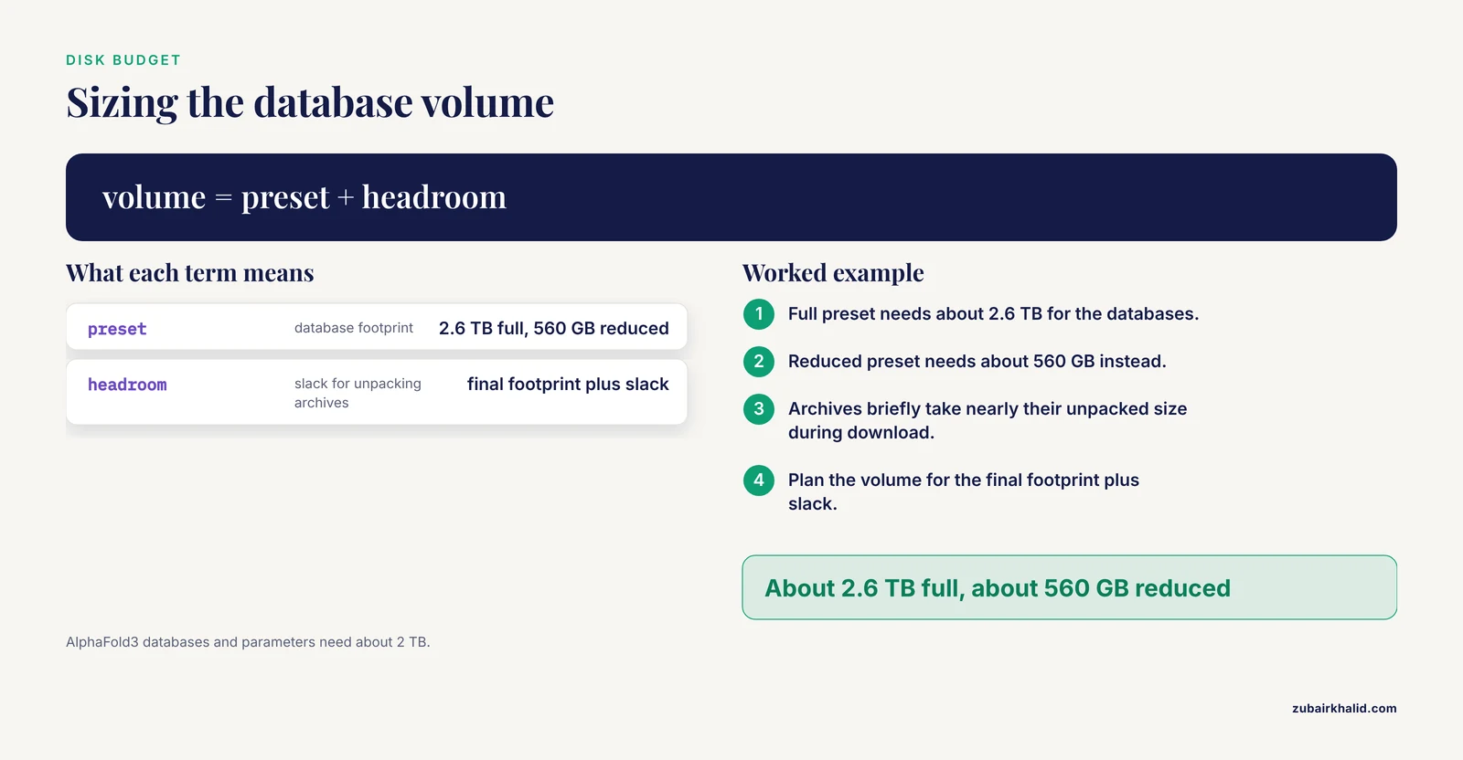
The databases want their own volume, sized to the preset you chose plus working headroom: about 560 GB for the reduced AlphaFold2 preset, about 2.6 TB for the full preset, and about 2 TB for AlphaFold3's databases and parameters. Archives consume nearly their unpacked size transiently during download and verification, so plan the volume for the final footprint plus enough slack that the unpacking stage never wedges against the quota. Outputs want a separate volume from databases, because their growth pattern is different: MSAs accumulate many files per prediction, and batch work generates output volume that surprises people who sized for the models alone.
Read-only discipline
Once the databases are downloaded and verified, make the directory read-only for users. This prevents the most annoying class of accident, where a misconfigured run writes into the database tree, and it also means multiple users and multiple containers can share one database copy safely. The bind-mount with :ro shown in the SLURM example enforces this at the container level.
What to archive and what to delete
A completed prediction directory contains ranked models, score JSON files, PAE and pLDDT images, the MSA directory, and timing logs. The models and scores are small and should be kept indefinitely. The MSA directory is the bulk of the size; keep it if there is any chance of rerunning model stages with different settings, archive it to cold storage if the project is dormant, and delete it only when you are confident the sequences will not be revisited. Rebuilding an MSA costs a full search cycle, which is exactly what you built the local pipeline to avoid repeating.
Versioning, Reproducibility, and Upgrades
AlphaFold is a moving target in a way that traditional command-line bioinformatics tools are not, because three components move independently: the model code and weights, the databases, and the container stack. A reproducibility strategy has to pin all three.
Pinning the stack
Record the container image digest, not just the tag, because tags are mutable. Record the model weights version directory. Record the database snapshot identifiers printed by the download scripts, which the main article's healthy-download output illustrates with versioned names such as the UniRef90 and MGnify releases shown there. For MSA service routes, record the date of the query, since the underlying databases behind a public API change without notice. None of this requires special tooling; a plain text file per experiment is sufficient, and the discipline matters more than the format.
When to upgrade and when to freeze
Upgrade deliberately, not automatically. A new model weights release can change predictions for the same input, which is a scientific event worth handling like a method change: rerun a small benchmark panel of proteins you know well, compare old and new outputs, and only then switch your production pipeline. Between upgrades, freeze the container image and databases so that a mid-project rerun reproduces the mid-project result. For papers, the frozen combination used for the final figures should be preserved until publication and ideally beyond.
Comparing across predictors
Version discipline becomes even more valuable when results from multiple predictors enter the same analysis. Because ABCFold treats results from AlphaFold 3, Boltz-1, and Chai-1 in a unified fashion and installs the alternative predictors at runtime as needed, it provides a natural frame for versioned cross-method comparisons, with visualization options that include steric clash information [2]. If your lab runs cross-method evaluations, adopt the same pin-and-record discipline across all the tools in the comparison, because a version mismatch between predictors is indistinguishable from a genuine method difference in the outputs.
Licensing and Terms of Use Considerations
The licensing asymmetry between AlphaFold2 and AlphaFold3 catches people by surprise, so it deserves its own section rather than a buried note.
AlphaFold2's weights and code are openly available, and the local installation can be used broadly, including in commercial contexts subject to the licenses of the constituent components. AlphaFold3 is different: the model parameters are provided free of charge but under terms of use that restrict commercial applications, and obtaining them requires requesting access and agreeing to those terms before download [as described in the software stack requirements of the official repository documentation]. The practical consequence is procedural, not technical: for a local AF3 install, build in lead time for the access request, and have institutional counsel or a technology transfer office confirm that your intended use, particularly any industry collaboration or screening service, sits within the terms.
The same terms-based thinking applies to the hosted AlphaFold Server, which is offered for non-commercial use with job volume and input size limits. A lab that starts on the server and later scales into commercial work cannot simply assume the same usage remains permitted; that is the moment to revisit the local installation route, with its own licensing review.
For the wrapper ecosystem, ABCFold is distributed as open scripts and documentation on GitHub and PyPI and installs with a standard pip install ABCFold, but each underlying predictor it wraps carries its own terms, so a multi-predictor comparison inherits the most restrictive license among them [2]. When in doubt, the terms of the individual model weights, not the wrapper, are what govern.
Common Misconceptions About Local Installation
Several beliefs circulate persistently in lab meetings and online forums. Each is worth correcting explicitly, because acting on any of them wastes real resources.
"I need the biggest GPU available." No. The documented baseline is 16 GB for monomer AlphaFold2 and an A100 40 GB is the recommendation for AF3 and comfortable multimer work. A GPU larger than that adds little for standard inputs. Money is usually better spent on disk for the full databases and on CPU cores for the search stage, which are the actual bottlenecks in batch work.
"Templates are required for a good prediction." As the main article notes, the MSA carries most of the signal for folded proteins. Templates help MSA-poor families and specific benchmarking scenarios. Installing the template databases is part of the standard setup anyway, but a missing or outdated template set is rarely the explanation for a poor model.
"If the structure looks right, the prediction is right." Visual plausibility is the weakest evidence available. AlphaFold models are almost always visually plausible; that is precisely why the confidence metrics exist and why screening-scale studies needed purpose-built evaluation, including the blind-screening design with a large excess of non-binders that exposed specificity limitations for SLiM detection and motivated an adaptive threshold [1]. Judge predictions with the metrics, in the reviewer's checklist above, and validate discovery claims experimentally.
"The installation is the hard part; after that it just works." The installation is the bounded, well-documented part. The unbounded parts are MSA quality for hard targets, metric interpretation for unusual inputs, and pipeline hygiene for batch work. Budget your effort accordingly.
"CPU-only is a viable fallback for real work." It is documented as possible for AlphaFold2 with GPU relax disabled, but a single monomer can take many hours to days and multimer jobs are effectively impractical. CPU-only is a contingency for verifying that a pipeline runs, not a production mode.
"A hosted server and a local install are interchangeable." They overlap on the simplest cases and diverge everywhere else. Local installs offer custom MSAs, batch throughput, template control, and reproducibility against frozen databases; the hosted server offers zero infrastructure. The hosted path has also been validated in the literature for specific workflows: the SLiM evaluation study used ColabFold as its practical route and presented a cost-effective workflow requiring no local installation for that screening task [1], which shows hosted routes can support real published science when the question matches their constraints. Match the route to the question rather than assuming either is universally sufficient.
Practical Applications: What Labs Actually Use Local AlphaFold For
Closing the loop from requirements to science, it helps to see where local installations deliver value that hosted services cannot, because this is the justification for the hardware and the terabytes.
Structural proteomics and annotation. Labs predicting structures for many proteins from an organism of interest use local batch pipelines with frozen databases so that every annotation in a paper comes from the same reproducible configuration. This is the canonical use case for the full-database route.
Complex and interface modeling. Multimer predictions of known complexes, with ipTM and PAE examination, support mechanistic papers where the interface architecture matters. Local control matters here because interface questions often require custom MSAs per chain and repeated reruns as constructs are redesigned.
Ligand and nucleic acid contexts. With AF3's JSON inputs, labs model protein-small molecule and protein-nucleic acid arrangements, and wrappers such as ABCFold make it routine to ask the same standardized question of AF3, Boltz-1, and Chai-1 and compare the answers, including steric clash visualization in the results [2]. Cross-predictor agreement is becoming an expected sanity check in this space, and it is practical only with local installs.
Motif and peptide screening. Short linear motif discovery against folded domains is an active application area, and the methodological literature has already shaped how it should be done: ColabFold-based workflows requiring no local installation for the screening itself, MiniPAE as the screening metric of choice, and adaptive thresholds to handle the unbalanced, non-binder-dominated reality of screening datasets [1]. A lab doing this at scale may still maintain a local installation for the follow-up structural characterization while running the screen itself on the lighter hosted route.
Method development and benchmarking. Anyone evaluating prediction methods, including new scoring approaches, needs the template-leakage control that max_template_date provides and the full preprocessing stack that hosted services abstract away. This is the use case where the local installation is not merely convenient but required for sound methodology.
The through-line across all of these is control. The local installation exists for the predictions where input format, database version, MSA provenance, or throughput requirements exceed what a hosted service offers. If none of those pressures apply to your current question, the lighter routes in this article, from ColabFold to the AlphaFold Server, will get you a structure today, and you can defer the terabyte download until your science actually demands it.
Frequently Asked Questions
Can I run AlphaFold without a GPU?
Yes for AlphaFold2, but only for very occasional use, because CPU-only inference of a single monomer can take many hours to days and multimer jobs are effectively impractical. Plan on an NVIDIA GPU with at least 16 GB of memory for real work.
How much disk space do I need for a local AlphaFold installation?
About 560 GB for the reduced AlphaFold2 database preset and about 2.6 TB for the full preset, plus under 100 GB for the container and model weights. AlphaFold3 needs roughly 2 TB for its databases and parameters.
What is the difference between the AlphaFold server and a local installation?
The AlphaFold server runs AlphaFold3 on Google-hosted hardware for non-commercial use with job and input-size limits, while a local installation gives you unlimited runs, custom MSAs, batch processing, and full control over templates at the cost of hardware and several terabytes of databases.
Can I install AlphaFold without downloading the large databases?
Yes. Wrappers such as ABCFold can generate MSAs through the MMseqs2 API instead of the local JackHMMER databases, letting AlphaFold 3 run locally with a far smaller footprint, with the tradeoff of depending on a remote MSA service [2].
What input file format does AlphaFold require?
AlphaFold2 takes FASTA files, one entry per chain for multimer jobs. AlphaFold3 takes a JSON job specification that encodes proteins, nucleic acids, ligands, and modified residues together, and both accept precomputed A3M or Stockholm MSAs to skip database searching.
Do I need structural templates for a good prediction?
No. The MSA carries most of the signal for folded proteins, and templates mainly help for MSA-poor families, though custom templates are supported and useful when you have an unpublished related structure.
How do I know whether my predicted structure is trustworthy?
Check the mean pLDDT, the PAE matrix, and, for complexes, the ipTM score. For short peptide binding questions, MiniPAE was reported as the most suited metric for SLiM screening [1].
Can I install AlphaFold on Windows or macOS?
Not natively. AlphaFold targets Linux. On Windows use WSL2 with CUDA passthrough, and on macOS there is no supported GPU path, so use the AlphaFold server, ColabFold notebooks, or a remote Linux machine instead.