How to Build Buffer Time into Your Thesis Timeline
By Dr. Zubair Khalid, DVM, MS, PhD ·

By the end of this article you will be able to build a quantitative buffer into your thesis timeline, a reserve of unplanned time that absorbs delays without pushing your defense past the deadline. You will calculate three duration estimates for every major task, combine them into an expected timeline, and size a buffer that matches how uncertain your work actually is. You will also get a worked example for a two-year biology thesis, a spreadsheet version you can copy, and a list of the mistakes that make buffers fail.
Here is what you need on hand before you start:
- A list of the major tasks in your thesis, from literature review through defense
- A realistic best case, most likely case, and worst case duration for each task (guess is fine, ten minutes per task is enough)
- A spreadsheet such as Google Sheets or Excel, or Python 3 installed on your computer
- Your institutional deadlines, especially the last possible defense date and any committee paperwork cutoffs
Nothing else is required. The math uses only addition, subtraction, multiplication, and a square root.
Why Thesis Timelines Fail Without a Buffer
Most thesis plans are built from single-point estimates. You write "data collection, 28 weeks" next to one task and "results chapter, 8 weeks" next to the next. The problem is that a single number hides two different things at once: the duration you expect, and the range of durations you could plausibly get. A cell culture line that keeps getting contaminated, a sequencer queue that runs three weeks long, a reviewer who takes two months instead of two weeks. None of these is unusual. Together they are why so many students defend months after their original plan.
Two planning ideas fix this:
- Separate task estimates from schedule protection. Each task gets an honest estimate of expected duration. The safety margin lives in one visible block of time at the end of the plan, not scattered in hidden padding inside every task.
- Size the buffer to the uncertainty, not to a feeling. A task with a narrow range of plausible outcomes needs almost no protection. A task with a wide range, like animal work or sample collection that depends on seasonal and equipment factors, needs a lot. You can measure that range instead of guessing at it.
This approach comes from established project management methods. The three-point estimate and the PERT expected value formula are standard material in operations research and project management textbooks, and the idea of concentrating safety time into a project buffer is the core of the critical chain method described by Goldratt and refined in later project scheduling literature. You do not need to read any of that to use the calculator. The formula is four lines long.
The Thesis Timeline Buffer Calculator Formula
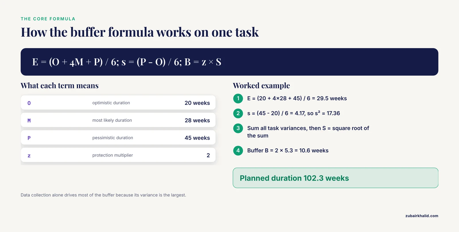
The calculator rests on two formulas applied to every task, followed by one formula for the buffer itself. This is the core of any thesis timeline buffer calculator formula.
For each task you supply three numbers, in weeks:
- O, the optimistic duration, if everything goes right
- M, the most likely duration
- P, the pessimistic duration, if reasonable things go wrong
Then:
Expected duration of a task:  E = (O + 4M + P) / 6
Uncertainty of a task:        s = (P - O) / 6
The first line is the classic PERT weighted average. It leans toward the most likely value but pulls the estimate up when the pessimistic case is far away. The second line measures how spread out your three estimates are. A routine writing task might have O = 6, P = 10, giving s = 0.67. A field season might have O = 12, P = 30, giving s = 3. The math sees the second task as roughly four and a half times riskier.
For the whole plan:
Expected timeline:  T = sum of all task E values
Total uncertainty:  S = square root of the sum of all task s² values
Buffer:             B = z × S
Planned duration:   T + B
The sum of variances, not the sum of the s values, is the statistically correct way to combine independent risks. Tasks that can slip at the same time partially cancel each other out, so adding the raw uncertainty values would overstate your buffer. The square root of the summed variances gives the combined standard deviation of the full timeline.
The multiplier z sets how much protection you buy:
| z value | Rough meaning | Use when |
|---|---|---|
| 1 | Timeline holds in about 8 of 10 realistic scenarios | You have a flexible defense window and an understanding committee |
| 1.65 | Timeline holds about 19 times out of 20 | A soft deadline with some flexibility |
| 2 | Timeline holds in the large majority of scenarios | A hard registration deadline, funding cutoff, or visa date |
These coverage figures follow from the normal distribution, which is the standard approximation behind this method. Most students planning around a hard graduation date should use z = 2.
How to Calculate Your Thesis Timeline Buffer: Step by Step
This walkthrough shows the full calculation in Python. If you prefer a spreadsheet, the next section gives the same result with formulas.
Step 1. List every major task with three estimates
Break the thesis into tasks of roughly two to ten weeks each. A biology thesis structure that works well for this purpose is:
- Literature review and proposal
- Methods development or protocol optimization
- Data collection (often the largest block, sometimes split into experiments)
- Data analysis and statistics
- Results chapter
- Discussion chapter
- Advisor review and revision
- Committee review and revisions
- Defense preparation
If your program expects a dissertation with multiple data chapters, treat each data chapter as its own line. If your thesis follows the classic five-chapter structure, the list above maps onto it directly.
For each task, write O, M, and P. A good habit: make P the duration that would still let you finish if the delay happened, not the disaster scenario. If a task slipping by a year means you change projects entirely, that risk belongs in your limitations discussion, not in the calculator.
Step 2. Enter the tasks into a Python script
Save this script as buffer.py and replace the numbers with your own.
from math import sqrt

# (task name, optimistic O, most likely M, pessimistic P) in weeks
tasks = [
    ("Literature review and proposal", 8, 10, 14),
    ("Protocol optimization",          6,  9, 16),
    ("Data collection",               20, 28, 45),
    ("[Statistical analysis](/blog/guides/statistical-analysis)",           6,  8, 12),
    ("Results chapter",                6,  8, 12),
    ("Discussion chapter",             6,  9, 14),
    ("Advisor review and revision",    4,  6, 10),
    ("Committee review and revisions", 4,  6, 12),
    ("Defense preparation",            2,  3,  5),
]

expected_total = 0.0
variance_total = 0.0

print(f"{'Task':<34}{'Expected':>10}{'s^2':>8}")
for name, o, m, p in tasks:
    e = (o + 4 * m + p) / 6
    s2 = ((p - o) / 6) ** 2
    expected_total += e
    variance_total += s2
    print(f"{name:<34}{e:>10.1f}{s2:>8.2f}")

sigma = sqrt(variance_total)
z = 2  # protection level, see table in the article

print()
print(f"Expected timeline:          {expected_total:.1f} weeks")
print(f"Combined uncertainty (S):   {sigma:.1f} weeks")
print(f"Buffer (z = {z}):             {z * sigma:.1f} weeks")
print(f"Planned duration:           {expected_total + z * sigma:.1f} weeks")
Step 3. Run it and read the output
python3 buffer.pyWith the numbers above, the expected output is:
Task                              Expected     s^2
Literature review and proposal       10.3    1.00
Protocol optimization                 9.7    2.78
Data collection                      29.5   17.36
Statistical analysis                  8.3    1.00
Results chapter                       8.3    1.00
Discussion chapter                    9.3    1.78
Advisor review and revision           6.3    1.00
Committee review and revisions        6.7    1.78
Defense preparation                   3.2    0.44

Expected timeline:          91.7 weeks
Combined uncertainty (S):   5.3 weeks
Buffer (z = 2):             10.6 weeks
Planned duration:           102.3 weeks
Step 4. Interpret the result
The expected timeline is about 92 weeks, roughly 21 months. The buffer adds another 10.6 weeks, about two and a half months. Your calendar plan should say you defend in roughly 104 weeks, and the final 10 to 11 weeks are marked as buffer, not assigned to tasks.
Two features of this output deserve attention. First, data collection dominates everything. Its variance term, 17.36, is larger than all the other tasks combined, so the size of your buffer is driven almost entirely by how honest you are about that one task. Second, the buffer is about 11.6 percent of the expected timeline, not the flat 25 percent many guides recommend. That is because most of the tasks in this example have fairly tight estimate ranges. If your pessimistic estimates are wider, your percentage will be larger, and that is correct behavior, not a bug.
Step 5. Place the buffer on the calendar
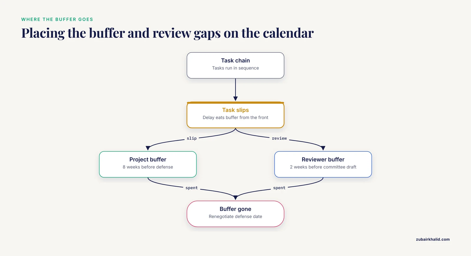
Buffer is not a task. It is unassigned time, and it works best split into two pieces:
- A project buffer of most of the total, placed immediately before your defense date, protecting the whole chain
- A small reviewer buffer of one to two weeks before each external review point (advisor draft, committee draft), because review turnaround is outside your control
For the worked example, that might be an 8-week project buffer before the defense and a 2-week gap before the committee sees the near-final draft. If a task slips, the slip eats the buffer from the front. When the buffer is gone, you still have the committee review window, and after that you are renegotiating your defense date.
Spreadsheet Version of the Calculator
If you would rather not run Python, this is how to calculate a thesis timeline buffer in a spreadsheet. Set up six columns:
| Column | Content | Formula (row 2, fill down) |
|---|---|---|
| A | Task name | typed |
| B | Optimistic (O), weeks | typed |
| C | Most likely (M), weeks | typed |
| D | Pessimistic (P), weeks | typed |
| E | Expected duration | =(B2+4*C2+D2)/6 |
| F | Variance | =((D2-B2)/6)^2 |
Then in summary cells below the table:
Expected timeline:   =SUM(E2:E10)
Total variance:      =SUM(F2:F10)
Buffer (z = 2):      =2*SQRT(SUM(F2:F10))
Planned duration:    =SUM(E2:E10)+2*SQRT(SUM(F2:F10))
These are the same formulas as the Python script, so the outputs match exactly. Enter your three estimates, and the sheet does the rest. Keep the z multiplier in its own cell, say H2, and reference it with =H2*SQRT(SUM(F2:F10)) so you can change your protection level without editing formulas.
A Worked Example Against Real Deadlines
Numbers in weeks mean little until they touch a calendar. Suppose your graduate program requires defense completion by May 15 and you start planning in August, giving you about 88 weeks. The worked example above needs 102.3 weeks at z = 2. That tells you immediately that the plan as estimated does not fit, and you have three honest options:
- Cut scope. Drop the third data chapter, or narrow data collection from three experiments to two. Re-run the calculator with the smaller task list.
- Compress estimates deliberately. Shift some tasks' M values down only if you have a concrete reason, such as a pilot dataset already in hand. Never compress just to make the deadline fit, because that silently deletes your protection.
- Negotiate the date. Many programs allow a defense in the following term. If your funding or visa permits, an honest plan with a buffer beats a fragile plan that hits the exact deadline.
The calculator earns its keep here. Instead of discovering the shortfall in March of your final year, you discover it in August, when you can still act.
A second use is backward scheduling from the defense date. Take the planned duration, subtract the buffer, and you get the latest reasonable start date for each chain of tasks. In the example, defense prep must begin no later than about 5 weeks before the defense, committee review must go out roughly 13 weeks before, and so on backward up the chain. Writing these trigger dates into your calendar turns the plan into a set of alarms.
Checking Your Numbers
Sanity checks that catch most input errors:
- P must be greater than M, and M greater than or equal to O, for every task. If not, your estimates are inconsistent. The Python script will still run and produce a smaller variance, which is the symptom to look for.
- The buffer should land between roughly 10 and 30 percent of the expected timeline for a typical thesis task list. A value outside that range usually means one task has wildly inflated P, or every task does. Look at the s² column and find the outlier.
- Add up your weeks and compare against the calendar. Weeks of planned work should account for most of the calendar time available, minus holidays, teaching weeks you already know about, and the buffer. If planned work is 91.7 weeks in an 88-week window, the mismatch is real regardless of how you feel about it.
- Re-run the calculator whenever a task finishes early or late. Update the finished task to its actual O = M = P value, re-estimate the remaining tasks, and check whether the remaining buffer still covers the remaining uncertainty. This takes five minutes and is the single highest-value maintenance habit for a multi-year plan.
Common Mistakes and Limitations
Hiding the buffer inside tasks. If every task quietly carries an extra 20 percent, you will spend that padding, lose track of it, and still miss the deadline. The buffer works because it is visible, separate, and the last thing to be spent.
Spending the buffer as soon as it exists. A buffer is not free time for a side project or a conference you have not budgeted. It exists to absorb real delays. Students who treat it as slack almost always need it later.
Optimistic most-likely estimates. The formula assumes your three numbers are honest. The most common failure is setting M to what the task would take if nothing went wrong, which makes P look absurdly far away and inflates the buffer to compensate. A better habit: M is the duration you would bet on, O and P describe the spread around that bet.
Forgetting fixed external delays. Committee members travel. Institutional review boards meet on set dates. Animal protocols renew on anniversary dates. Put known fixed waits in your task list as tasks with O = M = P, since they carry no uncertainty but do consume calendar time.
Ignoring concurrent work. The calculator assumes tasks run one after another. If you write your discussion chapter while the last experiment runs, the parallel tasks no longer simply add. For a first pass, model tasks as sequential, which is conservative and safe. If you want to model overlaps, subtract the overlapped weeks from the total expected duration manually and accept that the buffer becomes approximate.
Treating the output as a promise. The percentages attached to each z value come from a statistical model of your estimates, not from your actual future. The model is far better than a flat guess, but it inherits every error in your three-point estimates. Re-estimating as you go is what keeps it honest.
Skipping the human limits. A calculator cannot know that your advisor is on sabbatical next spring, that your program requires an intent-to-defend form six weeks ahead, or that your specific committee answers email slowly. Ask your graduate coordinator about every fixed administrative deadline in your program, then add them as tasks. And as with any plan, individual circumstances vary, so treat your advisor and committee as the authority on program-specific requirements.
Frequently Asked Questions
What is a thesis timeline buffer?
A thesis timeline buffer is a block of unplanned time placed at the end of your schedule, sized to absorb realistic delays without moving your defense date. It is calculated from the spread between your optimistic and pessimistic task estimates rather than chosen as an arbitrary percentage.
How do I calculate a buffer for my thesis timeline?
Estimate an optimistic, most likely, and pessimistic duration for each task, compute each task's expected duration as (O + 4M + P) / 6 and its uncertainty as (P - O) / 6, then multiply the square root of the summed uncertainties squared by 2 for a hard deadline. The Python script and spreadsheet formulas in this article do this for you.
How much buffer time is enough?
For most thesis plans a buffer between 10 and 30 percent of the expected timeline is appropriate, with the exact value driven by how uncertain your riskiest task is. Use z = 2 when defending against a hard deadline and z = 1 when your defense window is flexible.
Should I tell my advisor the buffer exists?
Yes. A visible buffer reads as a professional project plan, while a hidden one reads as padded estimates. Tell your advisor which weeks are reserve time so a delay can be discussed as buffer consumption rather than as the plan failing.
What happens if my buffer runs out?
When the buffer is exhausted, the next protection layer is the review window before your committee sees the draft, and after that your options are scope reduction or moving the defense date. If the calculator shows the buffer is spent early, act immediately rather than hoping later tasks run fast.
Does buffer planning work for lab-based biology theses?
Yes, and it matters most there. Lab and field work have the widest gap between optimistic and pessimistic outcomes, so those tasks dominate the buffer size. Model a long data collection phase as several separate experiments rather than one task, because independent experiments partially offset each other's delays.
How do I plan around a fixed defense date?
Work backward from the date. Subtract the buffer and each task's expected duration in reverse order to get a latest-start date for every task, and put those dates in your calendar as alarms. If the backward schedule starts before today, you must cut scope or renegotiate the date now.
Can I use this method for a dissertation or a course research project?
Yes. The method scales with the number of tasks, so the same formulas cover a one-semester project and a multi-chapter dissertation. For very short projects, use weeks as the unit of time throughout and keep the z = 1 setting unless a hard deadline applies.