Reproducible Research with Open Data
By Dr. Zubair Khalid, DVM, MS, PhD ·

By the end of this guide you will be able to take a public dataset, verify that the files you downloaded are the files the authors deposited, build an analysis that a stranger (or you, in two years) can rerun from scratch, and release your own data, code, and results so that others can do the same. You will need a computer with Python 3.10 or later or R 4.x, Git, a terminal, and accounts on a code hosting service such as GitHub and a data repository such as Zenodo or OSF. If you work with sensitive human data, you also need to know your institution's data sharing policy before day one, because it shapes what you can release and how.
Everything here applies whether you are reanalyzing published genomics data, linking environmental rasters to a health cohort, or building a predictive model on public chemistry data. The principles are the same. The details differ.
Why Reproducibility and Open Data Go Together
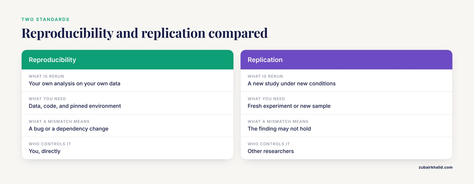
Reproducible research means that a competent person, given your data, code, and computing environment, can rerun your analysis and obtain the same numbers. Replication is a different standard. A replication study repeats the experiment under new conditions and asks whether the finding holds. Reproducibility asks a narrower question about your own pipeline. Both matter, but this guide focuses on the first because it is the one you control directly.
The case for building reproducibility in from the start is not abstract. Modern life science projects chain together many data transformations, and the more data volume and analytical complexity a project accumulates, the harder it becomes to trust the final result unless every step can be audited. Work on the learning health system, where routine clinical data feed research, quality improvement, and decision support, argues that reproducibility and auditability must be implemented throughout the workflow, and that data provenance technologies which automatically capture the trace of a research task and its resulting data are the practical way to do this [1]. The same logic applies to a single-person project on a laptop. If you cannot trace how a result was produced, you cannot reproduce it, and nobody can check whether it was produced correctly.
Open data makes this tractable. When the inputs are public, the only variables left in the reproducibility equation are your code and your environment, both of which you can pin down exactly. When you also release your outputs, the community gains datasets it can reuse in ways you never planned. The Personalized Environment and Genes Study illustrates the payoff. Researchers linked residential histories for 7,531 study participants with publicly available geospatial environmental data, built 88 geographic information system based exposure indicators, and tested them against 11 disease phenotypes using covariate-adjusted logistic regression, inverse probability of treatment weighted models, and LASSO regression. The approach surfaced associations complementary to a prior questionnaire based analysis, including links between air pollution and cardiovascular disease [2]. None of that scale would have been practical if the environmental layers had to be collected from scratch for each cohort.
What Counts as Open Data for Research
Open data for research is data published under a license that permits reuse, redistribution, and modification, in a format you can read without proprietary software. In the life sciences the standard sources include:
- Sequence archives such as NCBI GEO and SRA and the arrays and reads behind most published transcriptomics papers
- Structured knowledge resources such as UniProt for protein annotation
- Geospatial and remote sensing products, such as satellite imagery layers released as analysis ready surface reflectance data
- Repositories run by journals, funders, and institutions, including Zenodo, OSF, and figshare
Two properties matter more than the brand of the repository. First, the data must have a persistent identifier, ideally a DOI, so that citations keep working. Second, the deposit should carry documentation that lets you interpret every column. A CSV of unlabeled numbers is not open data in any useful sense. This is the same problem that motivated the Confero platform, which was built to store, in a comparable and long-term usable manner, the full list of genes with their associated statistical results, including differential expression values, t-statistics, and p-values, for each contrast of interest in transcriptomics experiments [3]. The lesson generalizes. Store the complete result set, not just the hits, and store it in a defined structure so downstream analyses and cross-study comparisons remain possible years later.
Formats matter as much as licenses. Tabular data should be CSV or Parquet rather than Excel, because Excel silently mangles gene symbols and dates. Raw instrument outputs, such as fluorescence curves or sequencing reads, should be archived as generated, with derived summaries in separate files. Container images and environment files travel with the code, not in a methods paragraph.
Set Up Your Workspace Once
Install the following before you touch any dataset. Doing this once removes most of the friction people blame on the data itself.
- Python 3.10 or later with the
pandas,numpy, andmatplotlibpackages, or R 4.x with thetidyverse. Install through Miniconda so environments are reproducible. - Git, available from the command line as
git. - A checksum utility. macOS and Linux ship with
md5sumorshasum. On Windows, use PowerShell'sGet-FileHash. - A text editor or IDE. VS Code and RStudio are the common choices.
- A data repository account (Zenodo, OSF, or your institutional repository) and a code hosting account (GitHub or GitLab).
Open Data for Research Step by Step
The following walkthrough covers a complete cycle, from finding a public dataset to publishing a rerunnable analysis. The commands are real and the expected outputs are shown where they matter.
Step 1: Define the Question and Pick a Dataset
Write your question in one sentence before you search. "Does residential exposure to air pollution associate with cardiovascular disease in cohort X" is answerable. "What can open data tell me" is not. Then search repositories for datasets that measure the relevant exposure and outcome. Read the data descriptor paper or README before downloading anything. Check three things: the license permits your intended use, the sample size fits your statistical plan, and the variables you need were actually collected.
A useful discipline is to write a short analysis plan at this stage, listing your outcome, exposures, covariates, and primary model. The exposome-wide association workflow mentioned above is a good template. That study defined its phenotypes and exposures in advance, then applied a consistent modeling strategy across all of them [2].
Step 2: Download and Verify the Data
Download files with a tool that records the source and date. From a terminal:
mkdir -p project/data/raw && cd project/data/raw
curl -L -o expression_matrix.csv "https://example-repository.org/dataset/files/expression_matrix.csv"
curl -L -o checksums.md5 "https://example-repository.org/dataset/files/checksums.md5"
md5sum -c checksums.md5
Expected output on success:
expression_matrix.csv: OKExpected output on failure:
expression_matrix.csv: FAILED
md5sum: WARNING: 1 computed checksum did NOT match
A failed checksum means the download is incomplete or corrupted, or that the repository changed the file after the checksum was published. Do not proceed. Redownload first. If it still fails, contact the data provider and record the correspondence in your project log. A checksum mismatch discovered six months later invalidates every result computed from that file, so catching it now is the cheapest quality control you will ever perform.
If the repository published file sizes and record counts, verify those too. For a CSV, a quick count is:
wc -l expression_matrix.csvStep 3: Record Provenance from the First Minute
Provenance is the record of where each piece of data came from and what was done to it. The research community has developed automated approaches to this, and experience from large distributed projects such as TRANSFoRm shows that capturing the trace of each research task enables both reproducibility and auditability across a workflow [1]. You do not need workflow middleware to benefit. A plain-text provenance log is enough for most projects, as long as you write it the day you download the data, not the week you submit the paper.
Create a file called data/PROVENANCE.md with this structure:
# Provenance Log

## 2026-11-11
- expression_matrix.csv downloaded from https://example-repository.org/dataset
- Version: v1.2, DOI: 10.0000/example.12345
- md5: a3f2...9c (verified OK against published checksums.md5)
- Original publication: Doe J et al. (2024)
- License: CC BY 4.0
- Notes: values are log2 normalized counts, 20,417 genes x 96 samples
Every script that transforms data should also write its own record. If scripts/01_clean.R converts raw counts to a filtered table, have it write data/processed/clean_meta.txt containing the input filenames, their checksums, the filtering parameters, and the session information. That habit mirrors what provenance-aware systems do automatically and gives you the audit trail without new infrastructure [1].
Step 4: Create a Pinned Computational Environment
Different package versions produce different numbers, sometimes dramatically so for statistical methods under active development. Pin your environment on day one.
With conda:
conda create -n openanalysis python=3.11 numpy pandas matplotlib scipy
conda activate openanalysis
conda env export > environment.yml
With R:
install.packages("renv")
renv::init()
renv::snapshot()
Expected output from renv::snapshot():
* Snapshot written to '/home/you/project/renv.lock'The resulting environment.yml or renv.lock file lists exact package versions. Commit it to version control. Anyone rerunning your project installs from that file and lands on the same software stack. If you use tools that change at the operating system level, such as BLAS libraries that alter floating point results, a container built from a Dockerfile with a pinned base image removes that variable too.
Step 5: Organize the Project and Script Every Step
Use a fixed directory layout so collaborators can find things:
data/raw/files exactly as downloaded, never editeddata/processed/outputs of cleaning scripts, regenerable at any timescripts/numbered scripts,01_clean.R,02_model.py,03_figures.Rresults/tables and model outputsfigures/final plotsPROVENANCE.md,README.md, environment file
The rule that makes reproducibility real is this: nothing in data/processed/, results/, or figures/ is ever edited by hand. Every file there is the output of a script. If you want to change a result, you change the script and rerun it.
A minimal scripted analysis in Python looks like this:
import pandas as pd

df = pd.read_csv("data/raw/expression_matrix.csv")
summary = df.describe().T
summary.to_csv("results/summary_stats.csv")
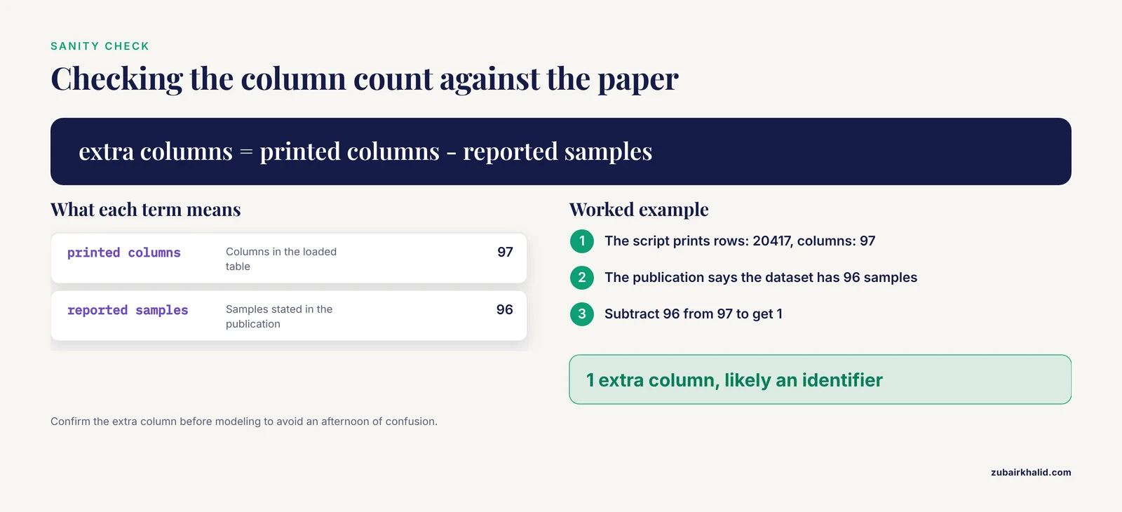
print(f"rows: {len(df)}, columns: {len(df.columns)}")
Expected output:
rows: 20417, columns: 97The printed line is your first sanity check. If the publication says 96 samples and you see 97 columns, the extra column is probably an identifier, and confirming that before modeling saves an afternoon of confusion.
For long projects, store intermediate statistical results in a defined, complete structure rather than as loose spreadsheet tabs. The contrast data model behind Confero, which keeps every gene with its effect size, t-statistic, and p-value for each contrast, exists precisely so that results from different studies and platforms can be compared computationally rather than by eyeballing figures [3]. Even a plain CSV with stable column names gets you most of that benefit.
Step 6: Version Control and Document
Initialize Git and commit early and often:
git init
git add scripts/ environment.yml README.md
git commit -m "Analysis pipeline v1: cleaning and summary statistics"
A common beginner error is trying to commit data files:
error: file 'data/raw/expression_matrix.csv' is large (412.3 MB)Large raw files belong in a data repository with a DOI, not in Git. Record the DOI and checksum in your README and provenance log instead. Add a .gitignore excluding data/raw/ and data/processed/ from the first commit.
Your README should let a stranger rerun everything. Include the download commands, the environment setup, the script execution order, and the expected runtime. If a single script takes four hours, say so. Silent surprises destroy trust faster than slow pipelines.
Step 7: Validate the Result
Before trusting your output, check it three ways. First, rerun the whole pipeline from a clean directory and confirm the final numbers match, to the last decimal place or within a stated numerical tolerance for parallelized operations. Second, reproduce at least one published number from the original paper as a benchmark. If the original authors reported a specific fold change or odds ratio and your pipeline cannot recover it from their data, either your environment differs from theirs or you have a bug, and either finding is worth knowing before you extend the analysis. Third, apply a domain sanity check. When a study links external data layers to a cohort, as in the geographic exposure work that built 88 indicators from open geospatial sources for 7,531 participants, the authors checked the resulting associations against prior questionnaire based findings from the same cohort and reported where the two approaches agreed and diverged [2]. Agreement is not proof, but divergence you cannot explain is a red flag.
Step 8: Publish Data, Code, and Model Artifacts
When the project ends, release the pieces. Push code to a hosting service, archive the repository on Zenodo to get a DOI, deposit data files with their checksums, and deposit the environment file. If your project produced a predictive model, follow the practice demonstrated by the Flame framework, an open source platform for building and hosting predictive models, which stores every model in a repository supporting versioning, identifies each model with a unique ID, and attaches detailed documentation formatted with widely accepted standards [4]. You can adopt the same discipline without the infrastructure. Give each trained model a version number, save the training data checksum, the environment file, the random seed, and the hyperparameters alongside the model object, and write a short card describing intended use and limitations.
Seeds deserve special mention. Set them explicitly and record them:
import numpy as np
np.random.seed(42)
An unrecorded seed makes stochastic methods, such as random forests and neural networks, irreproducible in practice even with identical data and code.
Worked Examples from Current Practice
Three recent projects show how these pieces combine in real life science.
The exposome study described above is a model of open data reuse. Its authors used open source GIS software to join public environmental layers with cohort residential histories, constructed the exposure indicator set, and ran a defined statistical pipeline across phenotypes [2]. The entire approach depends on data being open, and its design as a standardized, repeatable process is what makes it applicable to other cohorts.
The peatland assessment framework combining spectral and molecular data shows how open satellite imagery can anchor a multimodal study. Researchers derived spectral indices, including NDVI, EVI, gNDVI, Greenness Index, and albedo, from PlanetScope analysis ready surface reflectance data across nine European peatland sites spanning three climatic zones, then examined how those spectral signals corresponded with site level biogeochemical measurements, including elemental carbon and nitrogen contents and molecular composition from pyrolysis-GC/MS [5]. The spectral indices and the reflectance product are the open layer. The molecular measurements are the expensive layer. The design deliberately pairs the two so that the costly measurements calibrate a signal that can then be scaled widely.
QuantDSF shows the software side. Nano differential scanning fluorimetry workflows often reduce each experiment to a single melting temperature, discarding concentration dependence and temperature resolved binding information. QuantDSF, an open source platform, extracts thermal stability, affinity, and binding thermodynamics, reporting the melting temperature through three complementary algorithms and deriving apparent enthalpy and entropy via isothermal slicing and Van't Hoff regression, with validation against isothermal titration calorimetry and surface plasmon resonance [6]. Because the code is open, a reader can inspect exactly how each melting temperature was determined, which is impossible with a closed vendor pipeline that returns only a number.
Together these examples make the same point. Open inputs, scripted processing, transparent algorithms, and versioned outputs turn a one-off result into infrastructure.
Key Options at a Glance
| Decision | Common options | When to choose |
|---|---|---|
| Tabular format | CSV, Parquet | CSV for small, human-readable data. Parquet for large tables with mixed types |
| Data license | CC0, CC BY 4.0 | CC0 for maximum reuse, CC BY when attribution matters |
| Code license | MIT, Apache 2.0, GPL-3.0 | MIT for simplicity, GPL to require derivatives stay open |
| Environment pinning | conda environment.yml, R renv.lock, Docker image | conda or renv for most projects, Docker when system libraries matter |
| Checksums | MD5, SHA-256 | SHA-256 for new deposits, MD5 where providers publish only MD5 |
| Data deposit | Zenodo, OSF, institutional repository | Zenodo or OSF for general data, field specific archives for sequences and structures |
| Statistical result storage | Full result tables per contrast | Always. Keep every gene and every test, not only significant hits [3] |
Practical Tips
Write the README first. If the instructions are unclear while you still remember the details, they will be useless in a year.
Keep raw data read-only at the file system level with chmod -R a-w data/raw/ so accidental edits fail loudly instead of silently.
Name scripts by execution order. 02_model.py running before 01_clean.py is a bug you can see in the file list.
Log your session information in every result file. In R, sessionInfo(). In Python, print the versions of pandas, numpy, and scipy. A results table without this context cannot be compared across computers.
Prefer explicit file paths computed from a single project root variable over absolute paths containing your username, which break on every other machine.
Reproduce one published result before extending an analysis. It validates your environment, your reading of the data documentation, and your pipeline in a single pass.
Record model versions and parameters as Flame does, with unique identifiers and standards-based documentation, so collaborators can cite a specific model rather than "the model from around March" [4].
Common Mistakes and Limitations
Cleaning raw files by hand. Opening a CSV in Excel, deleting two rows, and saving destroys the link between the deposited data and your analysis. All cleaning belongs in scripts that read from data/raw/ and write to data/processed/.
Treating a notebook as the record. A Jupyter notebook run top to bottom out of order, twice, produces a state nobody can reconstruct. Notebooks are fine for exploration. Before release, restart the kernel and run every cell in order, or convert the logic into plain scripts. An unexecuted notebook with saved outputs is documentation, not an analysis.
Skipping the checksum. Unverified downloads are the most common silent failure in secondary data analysis. One md5sum -c per dataset removes the risk.
Confusing reproducibility with correctness. A pipeline can be perfectly reproducible and produce a wrong answer because the model was misspecified or the covariates were chosen after looking at the outcome. Reproducibility makes your work auditable. It does not certify the science.
Ignoring the license. Data released for research use may not permit commercial reuse or redistribution of derivatives. Check before you build a product on a public dataset, and cite the dataset itself, not only the paper describing it.
Overwriting processed data with no way back. If data/processed/ can be regenerated by rerunning the scripts, this is harmless. If it cannot, you have lost the pipeline. Test regenerability by deleting a processed file and rebuilding it early in the project, not after submission.
One inherent limit applies to any advice in this area. Projects involving human participants carry obligations, privacy constraints, and institutional review requirements that no generic checklist can resolve, and those constraints determine what you may share even when everything else argues for full openness. Plan around them from the start rather than discovering them at submission time.
A Reproducibility Checklist
Run this list before you publish, and ideally at each project milestone.
- Data files have a persistent identifier (DOI or accession) recorded in the README
- Downloaded files verified against published checksums, with the verification date logged
PROVENANCE.mdlists every input, its source, version, license, and checksum- Environment file (
environment.yml,renv.lock, or Dockerfile) committed to the repository - Every figure, table, and statistic regenerable by running scripts in documented order from
data/raw/ - Random seeds set in code and recorded in the README
- Session information captured in every results file
- Pipeline rerun from a clean directory with matching final results
- At least one published value reproduced as a benchmark
- Repository archived with a DOI, data deposited with checksums, models versioned with unique identifiers and documentation
- README tested by a colleague who reruns the analysis without your help
- Data use permissions and privacy constraints confirmed in writing
If you can tick all twelve, a stranger with a laptop and patience can rebuild your result, which is the entire point.
Frequently Asked Questions
What is the difference between reproducibility and replication?
Reproducibility means rerunning your analysis on your data with your code and getting the same numbers. Replication means conducting a new study that tests whether the original finding holds. A result can be perfectly reproducible and still fail to replicate.
Where can I find open datasets for life science projects?
Start with field-specific archives such as NCBI GEO and SRA for sequencing and expression data, structured resources such as UniProt for protein information, and general repositories such as Zenodo and OSF. Journal data availability statements are often the fastest route to the exact dataset behind a paper.
How do I cite a dataset properly?
Cite the dataset itself by its persistent identifier and version, in addition to the publication that describes it. Most repositories generate a ready-made citation text with author names, year, title, repository, and DOI that you can paste into your reference list.
What license should I put on my own data and code?
For data, CC0 maximizes reuse and CC BY 4.0 adds a mandatory attribution condition. For code, MIT is the simplest permissive option and GPL-3.0 requires derivatives to remain open. Choose one deliberately rather than leaving files unlicensed, because unlicensed material is legally unusable by others.
Do I need to share raw human data to be reproducible?
No. Privacy constraints can prevent raw data release. In those cases deposit the processed data, the full code, the environment specification, and as much metadata as your data use agreement allows, and state clearly what is withheld and why. Auditable code plus documented data processing still makes the analysis checkable.
How much data cleaning can I do before sharing?
Share the raw files exactly as you received them, alongside every cleaning script. Hand-edited files break the audit trail, because nobody can distinguish your corrections from your errors. If the original provider's files contain defects, document them and provide corrected versions as derived files.
What if the results change when I rerun the analysis?
First compare environments, because package version differences are the most frequent cause. Then check random seeds for stochastic methods. Small differences in floating point arithmetic can be tolerated with a stated tolerance. Large differences indicate a bug or a dependency change, and finding which is itself valuable science.
Is a computational notebook enough for reproducibility?
Not by itself. A notebook with saved outputs from an unknown execution order is documentation, not a rerunnable analysis. Restart the kernel, run all cells in order from top to bottom, verify the outputs match, and store the notebook with its environment file and data checksums before calling it reproducible.
Sources
- Embedding data provenance into the Learning Health System to facilitate reproducible research.
- Applying geographic information systems data linkages for an exposome-wide association study in the Personalized Environment and Genes Study.
- Confero: an integrated contrast data and gene set platform for computational analysis and biological interpretation of omics data.
- Flame: an open source framework for model development, hosting, and usage in production environments.
- Building a Framework for Peatland Assessment in Europe by Combining Spectral and Molecular Data.
- QuantDSF: an Open-Source Platform for Comprehensive Nano Differential Scanning Fluorimetry Analysis.