Power Analysis and Sample Size for Proportions
By Dr. Zubair Khalid, DVM, MS, PhD ·

A power analysis estimates the probability that a planned statistical test will detect a real effect of a stated size, and a sample size calculation runs that same logic backward to find the number of observations needed to reach a target probability, such as 80 percent.
Rule of thumb for proportions: with two independent groups, moderate sample sizes, and expected rates that stay away from 0 and 1, the classic normal approximation formula is accurate and fast. Move to exact or simulation-based methods when samples are small, events are rare, observations are clustered, or group sizes are unbalanced. If the goal is a confidence interval of a fixed width rather than a hypothesis test, plan with a precision-based calculation instead.
This guide defines the inputs behind every power analysis for proportions, compares the main options and their pros and cons side by side, shows where to run them, works through realistic scenarios, and lists the mistakes that most often sink a planned study.
The Four Inputs Behind Every Power Analysis for Proportions
A proportion summarizes a binary outcome, such as infected versus uninfected or responder versus nonresponder, as a fraction of trials. If 42 of 100 treated animals respond, the proportion is 0.42. Counts like this follow the binomial distribution, the model for the number of successes in a fixed number of independent trials that each carry the same success probability.
Four quantities are locked together, and fixing any three determines the fourth.
- Alpha (α), the significance level. The risk of declaring an effect real when it is only noise, called a Type I error. Most life science studies set alpha at 0.05.
- Power, written 1 - β. The probability of detecting an effect that truly exists. β is the Type II error rate, the risk of missing a real effect. Conventions are 0.80 for routine work and 0.90 when a miss would be costly.
- Effect size. The smallest difference worth detecting. For two proportions this can be the difference p1 - p2, the odds ratio (the ratio of the odds of the outcome in one group to the odds in the other), or Cohen's h, defined as h = 2 × arcsin(√p1) - 2 × arcsin(√p2), with values near 0.2 considered small, 0.5 medium, and 0.8 large.
- Sample size. The number of independent observations.
One structural feature of proportions drives everything else. Their variance is p × (1 - p), which peaks at p = 0.5 and shrinks toward the extremes. A study expecting 5 percent events faces different uncertainty from one expecting 50 percent, even with identical group sizes. For a single proportion tested against a fixed reference value, the same four inputs drive a one-sample version of the calculation.
Choosing the effect size is the hardest step. Three standard sources exist: pilot data from your own system, published estimates from comparable studies, and the minimal difference that would matter scientifically regardless of what the literature reports. Every assumed value is a guess, and the reporting review discussed below shows how often that guess turns out optimistic.
Software such as G*Power supports a priori mode (compute the required n from alpha, power, and effect size), post hoc mode (compute achieved power from a finished sample size), sensitivity mode (find the smallest detectable effect for a fixed n), and compromise mode (trade alpha against power) [1]. A priori is the mode you want at the planning stage.
Power Analysis and Sample Size Proportion Options at a Glance
Six approaches cover nearly every design involving proportions. The table compares them on the criteria that decide real choices.
| Option | Core assumption | Best for | Pros | Cons |
|---|---|---|---|---|
| Normal approximation (z-test) | The binomial behaves like a normal curve (large n, moderate p) | Two independent groups with moderate rates | One-line formula, transparent, available in every calculator | Unreliable for small samples, rare events, unbalanced allocation |
| Chi-square or likelihood-ratio framework | Large-sample approximation for cross-tabulations | 2×2 and larger tables, survey and genetic data | Matches the tests most analysts actually run, equivalent power under balanced allocation | Under unbalanced allocation, test choice changes power [2] |
| Exact binomial | Nothing beyond the binomial model | Small samples, rare events, one-to-one trials | Valid at any sample size and any rate | Conservative, needs more subjects for the same power, scarce in simple calculators |
| Model-based (generalized linear and mixed models, beta-binomial) | A stated mean-variance structure | Clustered, overdispersed, or covariate-adjusted proportions | Handles real data structure, robust effect-size measures exist [3] | Needs modeling skill, a wrong structure distorts power |
| Simulation (Monte Carlo) | Whatever you encode | Complex or nonstandard designs | Any design, any test, full flexibility | Requires programming, output is only as good as the encoded assumptions |
| Precision-based (confidence interval width) | Normal approximation for the interval | Estimation goals such as prevalence surveys | Fewer subjects, direct control of estimate quality | Can leave power near 50 percent if the result later feeds a decision [4] |
The Six Options Explained
1. Normal Approximation Formulas
The workhorse for two independent proportions. It treats the difference between two proportions as normally distributed, which is reasonable when each group contains enough successes and failures for the approximation to hold (a common working rule is at least 5 to 10 of each). For equal group sizes, the required number per group is:
n per group = (1.96 × √(2 × p × (1 - p)) + 0.84 × √(p1 × (1 - p1) + p2 × (1 - p2)))² ÷ (p1 - p2)²
where p is the average of the two expected proportions, 1.96 is the normal value for two-sided alpha of 0.05, and 0.84 is the value for 80 percent power.
Pros: transparent arithmetic, fast to sanity-check, and the default in nearly every calculator. Cons: the binomial distribution is skewed when p approaches 0 or 1, exactly where many biology studies live (rare adverse events, low infection rates), so the approximation can misstate power. A continuity correction, an adjustment that smooths the mismatch between a discrete distribution and a continuous curve, is applied by some software at analysis but not at design, creating a second mismatch. When expected rates fall below roughly 10 percent or above 90 percent, or when a group will contain fewer than about 30 observations, cross-check the result with an exact or simulation method.
2. Chi-Square and Likelihood-Ratio Frameworks
Analysts rarely compute a z-test by hand on a 2×2 table. They run Pearson's chi-square test or the likelihood-ratio test, and a power analysis should match that choice. These are asymptotic tests, meaning they rely on large-sample approximations, and comparative work shows the choice among them is not cosmetic. When the two groups are planned with equal sizes, Pearson chi-square, likelihood-ratio, and odds-ratio-based tests are equivalent in power. When allocation is unbalanced, their power can differ substantially, and the most powerful test depends on the actual proportions being compared [2]. The same research shows that when two proportions are compared only indirectly, through tag variables that stand in for the quantity of interest (as in genome-wide association studies), the power gaps widen as the tag variables weaken, one reason rare variant detection remains so difficult [2].
Pros: planning aligns with the test most software runs by default. Cons: under unbalanced allocation you must decide which test you will run, not just how many subjects you need. If cost or ethics push you toward unequal group sizes, run the calculation under the specific test and allocation you will actually use, not under a generic balanced assumption.
3. Exact Binomial Methods
Exact methods compute probabilities by enumerating the binomial distribution directly instead of approximating it with a normal curve. They stay valid at any sample size and any event rate, which makes them the right tool for small trials and rare outcomes. The price is conservatism: exact procedures often hold the true Type I error below the stated level, so they need somewhat larger samples for the same power, and many simple calculators do not offer them. Small animal transmission experiments, where each infectious-susceptible pair contributes a single binary outcome, are a case in point, and the worked scenario below shows what this demands in practice.
4. Model-Based Methods for Clustered and Overdispersed Proportions
Real proportion data often carry structure: multiple trials per subject, animals within pens, patients within clinics. Overdispersion means variability greater than the binomial model predicts, and it appears whenever outcomes within a cluster correlate.
Three planning routes cover this territory. Generalized linear models (GLMs) extend the proportion test to covariates, and quasi-likelihood versions relax the exact variance assumption. Methodological work shows that two GLM-based effect size measures, 2SLiP (two standard deviations in the linear predictor) and a pseudo-partial R-squared, extend directly to quasi-likelihood models and remain accurate when the variance function is misspecified, which protects the calculation against one of its most common failure modes [3].
For clustered binary outcomes, a simulation study in behavioral research compared linear regression, Poisson regression, beta-binomial regression, and generalized linear mixed models (GLMMs). GLMMs were powerful, beta-binomial regression outperformed them across a range of scenarios, linear regression was less powerful though its Type I error stayed near nominal, and Poisson regression was mostly anticonservative, meaning it produced more false positives than the stated alpha implies [5]. Plan the sample size under the model you will actually fit.
Cluster randomized designs, where whole units such as clinics or pens are assigned together, add a design effect of 1 + (m - 1) × ρ, where m is the average cluster size and ρ is the intracluster correlation coefficient, the share of variance shared by members of the same cluster. A palliative care trial planned at 20 units, 10 per arm with about 50 patient records per cluster per timepoint, illustrates the scale at which this inflation is designed in [6]. Ignoring it is among the fastest ways to lose power.
5. Simulation-Based Power Analysis
Monte Carlo simulation, meaning repeated random sampling, writes the design as code, generates many synthetic datasets under a stated effect size, runs the planned test on each, and reports the fraction that reach significance. That fraction is the estimated power. A minimal version has four steps.
- Fix the assumptions: group sizes, true proportions, clustering, and expected missingness.
- Generate many synthetic datasets, commonly 1,000 to 10,000, under those assumptions.
- Run the exact test you plan to use on each dataset.
- Divide the number of significant results by the number of datasets.
Poultry research offers a concrete template. Investigators reanalyzed broiler performance and quality trials by simulating them 1,000 times, then varied how many birds per pen were processed, from 5 up to 16 or 20 birds within pens of 18 to 27, to judge the sampling depth needed for weight, yield, and myopathy scoring [7].
Pros: any design, any test, clustered data, planned missingness, nothing is out of reach. Cons: you must program it, and the answer is only as trustworthy as the assumptions you encode. Report the generating assumptions alongside the resulting power.
6. Precision-Based Sample Size Determination
Precision-based planning targets the width of the confidence interval, the range of values the data support at a stated confidence level, rather than the power of a test. For a single proportion with target half-width d at 95 percent confidence:
n = 1.96² × p × (1 - p) ÷ d²
This route typically needs fewer subjects, and consumer and regulatory studies often take it because the deliverable is an estimate of how people behave, not a test against a threshold [4]. The catch is decision-making. Evaluations show that when the target precision is set equal to the gap between the expected proportion and the threshold that would count as a meaningful result, the design achieves only about 50 percent power, and the underpowering worsens when planners use a normal approximation at design time but an exact method at analysis [4]. Precision-based designs are well suited to description and risky for decisions.
Software, Calculators, and Where to Run the Numbers
Students and new researchers usually start by hunting for a biology calculator that handles power and sample size. Three tiers cover most needs.
G*Power is the standard free desktop program. Version 3.1.9.7 covers z-tests for proportions alongside t-tests, analysis of variance (ANOVA), correlation, and regression, and its a priori mode returns the required sample size from alpha, power, and effect size [1]. Its published workflows also catalog common pitfalls, which makes the documentation worth reading even if you compute elsewhere.
Scripted work belongs in R, where packages such as pwr provide functions for one- and two-proportion tests and base R runs simulations in a few lines. Design-specific web tools fill the gaps. The Non-Human Primate Sample Size Calculator at midas.wakehealth.edu covers 11 species and projects sample counts across longitudinal studies while accounting for natural deaths, a problem generic calculators cannot handle [8]. Methods papers increasingly ship their own tools, such as the R Shiny app accompanying a group-sequential method for comparing two survival probabilities at a fixed time point [9].
High-throughput settings need a bioinformatics calculator matched to the planned analysis. For DNA methylation arrays, simulations comparing six statistical approaches found that at very small samples (3 or 6 per group) the empirical Bayes and bump hunting methods delivered the highest power with controlled false discovery rate, the expected share of false positives among declared findings, when methylation sites were independent, while at 12 or 24 per group most methods converged [10]. A power number computed under one method does not transfer to another.
Whatever tool you use, record the tool, version, and inputs in the protocol so the calculation can be reproduced at analysis time.
Worked Scenarios
Scenario 1: Two Independent Groups
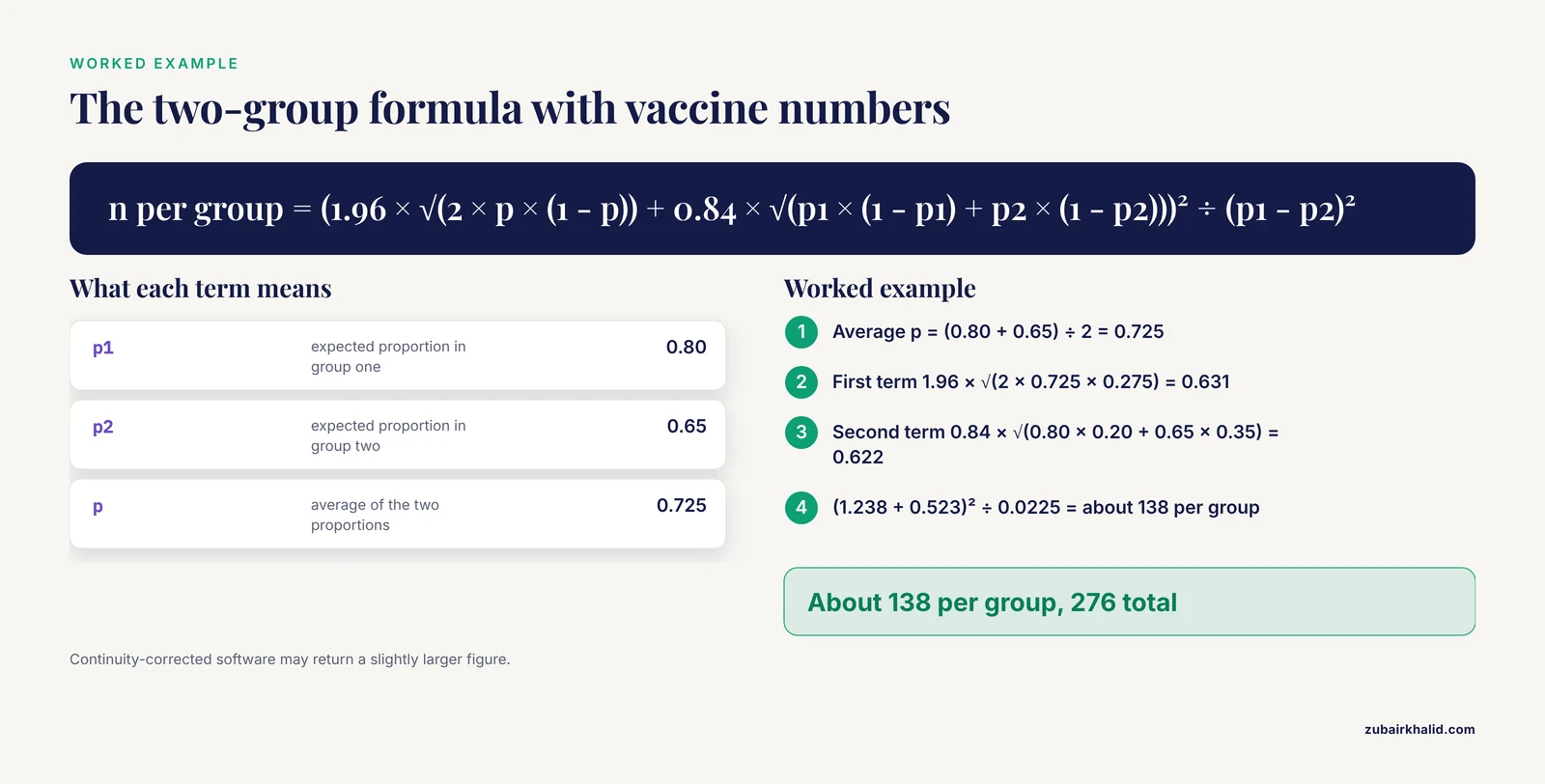
A lab is testing whether a new vaccine formulation raises the proportion of seroconverting mice (developing detectable antibodies) from 65 to 80 percent. Alpha 0.05 two-sided, power 0.80, equal groups.
n = (1.96 × √(2 × 0.725 × 0.275) + 0.84 × √(0.80 × 0.20 + 0.65 × 0.35))² ÷ (0.80 - 0.65)²
The two square root terms evaluate to 0.631 and 0.622, so the calculation is (1.238 + 0.523)² ÷ 0.0225, about 138 per group and 276 total. Software that applies continuity corrections may return a slightly larger figure. Add allowance for failed samples before ordering animals.
Scenario 2: Estimating a Single Proportion
A team wants to estimate the prevalence of a condition with a 95 percent confidence interval no wider than ±5 percentage points. With no prior information, the conservative choice p = 0.5 gives n = 1.96² × 0.25 ÷ 0.05², which rounds up to 385. If published studies suggest 10 percent, the same formula gives 139. Estimates get cheaper as the proportion moves away from 0.5, which is why even a rough pilot estimate pays for itself. If the survey will also test whether prevalence exceeds a threshold, revisit the 50 percent power warning in the precision-based option.
Scenario 3: A Small Transmission Study
An influenza group compares transmissibility between two virus strains in ferrets using one-to-one pairs. The outcome per pair is binary, so the analysis compares two proportions with tiny numbers. Published guidance for this design is at least 4 pairs per group for a two-group comparison, together with the observation that 3 infected pairs out of 3 still cannot establish transmissibility above a basic reproduction number (R0, the average number of secondary infections per infected individual) of 1 [11]. At this scale the plan should be built on exact binomial calculations, and the effect size input should come from prior transmission data rather than optimism.
Scenario 4: A Paired Comparison of Proportions
When the same items are tested under two conditions, the proportions are paired and the analysis uses McNemar's test, which evaluates the discordant pairs, the cases where the two conditions give different outcomes. A study benchmarking three AI chatbots on 200 German medical exam questions was planned this way, with an a priori power analysis setting a minimum of 195 questions [12]. Paired designs remove between-subject variability and generally need fewer units than independent designs for the same power, but the calculation must be done on the discordant-pair scale, not the raw proportions.
From Raw Number to Final Sample Size
Treat the formula output as a floor. Three adjustments usually follow.
- Dropout and unusable samples. Divide by the expected fraction of usable observations. If 138 per group is required and 15 percent of samples fail quality control, plan 138 ÷ 0.85, about 163 per group.
- Rounding and allocation. Round up, and keep the planned allocation ratio, because unequal group sizes change power as described above.
- One-sided versus two-sided. A one-sided test halves the alpha burden and needs fewer subjects, but reserve it for effects whose direction is fixed in advance and declared in the protocol.
How to Choose the Right Option
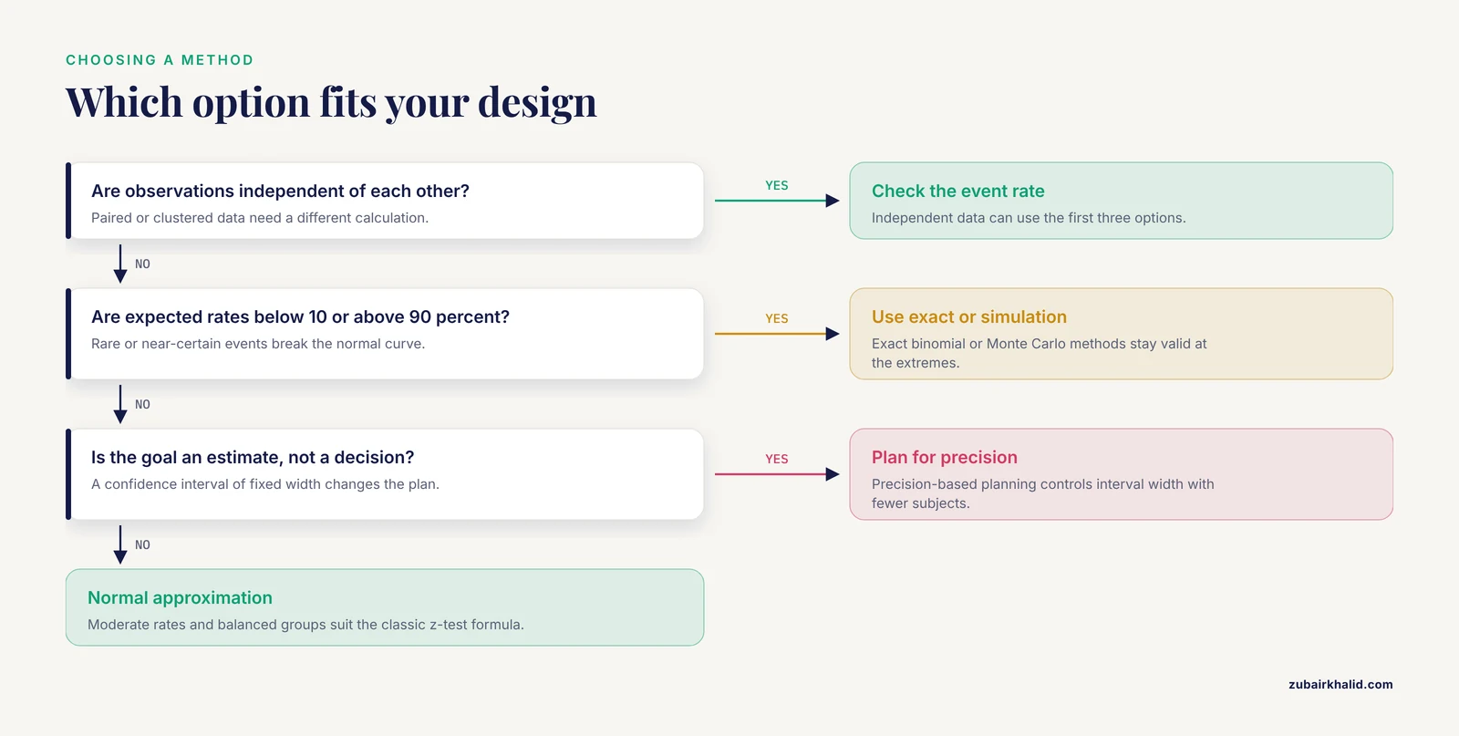
The pros and cons in the table reduce to six questions.
- Independent, paired, or clustered? Independent points to the first three options, paired to a McNemar-based calculation, clustered to model-based planning with a design effect.
- One proportion or a comparison? A single proportion with an estimation goal points to the precision-based option.
- Are the expected rates moderate? Below roughly 10 percent or above 90 percent, favor exact or simulation methods.
- Is allocation balanced? If not, decide which test you will run, because power differences between asymptotic tests become real [2].
- Will the result support a decision or only an estimate? Decisions need power-based planning.
- Are interim analyses planned? Each look at accumulating data inflates the Type I error unless the design and sample size are adjusted, and methods with error control across looks exist for binomial-style endpoints at a fixed time point [9].
There is no single best power analysis and sample size option for proportions. The right option is the one that matches the test you will run, the structure of your data, and the decision your study must support.
Common Mistakes and Limitations
Reporting gaps are common, and dichotomous outcomes fare worst. A review of 107 randomized trials across five orthodontic journals found that all essential planning parameters were reported for 62.1 percent of trials with continuous outcomes but only 41.6 percent of those with dichotomous or time-to-event outcomes, that roughly 55 percent of assumed sample sizes were smaller than recalculated values, and that about 30 percent of studies showed discrepancies above 10 percent [13].
Other recurring errors:
- Designing with one method and analyzing with another. A normal-approximation plan paired with an exact analysis delivers less power than the plan promised [4].
- Trusting the normal curve at the extremes. Rare events and small groups break the approximation precisely where it is most tempting to use.
- Ignoring clustering or overdispersion. Treating correlated outcomes as independent inflates the effective sample size and the false positive rate, a pattern documented across methods for clustered binary data [5].
- Forgetting dropout and missing data. Complete-case analysis, which discards records with missing values, can bias results and reduce power, while imputation methods preserved power across missingness patterns in simulation work spanning 10 to 50 percent missing values [14]. Inflate the planned number accordingly.
- Unbalanced allocation without a test-choice decision.
- Post hoc power as evidence. Power computed after a nonsignificant result largely restates the p-value, the probability of a result at least this extreme when no effect exists, and proves nothing about whether the effect is absent.
- Wishful effect sizes. The calculation is only as good as the assumed proportions. Ground them in pilot data or published estimates, and report the assumptions next to the result.
- Multiple testing. Testing many proportions at once inflates the false positive burden, and alpha adjustments raise the required n, which is why high-throughput screens plan around false discovery rate control instead [10].
One limitation deserves a line of its own. Alpha 0.05 and power 0.80 are conventions, not laws, and any individual study, especially one with ethical or cost constraints, benefits from a statistician's review before data collection begins.
Frequently Asked Questions
What is the difference between a power analysis and a sample size calculation?
A power analysis estimates the probability that a planned test will detect a stated effect with a given sample size, while a sample size calculation runs the same logic backward to find the number of observations needed for a target power. Both share the same inputs, alpha, power, and effect size.
How many subjects do I need to compare two proportions?
There is no universal number. The requirement depends on alpha, power, and the gap between the two expected proportions. In the worked example of 80 versus 65 percent with two-sided alpha of 0.05 and 80 percent power, the need is about 138 per group, and smaller gaps require far more.
When should I avoid the normal approximation for proportions?
Avoid it when samples are small, when expected proportions fall below roughly 10 percent or above 90 percent, or when group sizes are unbalanced. Exact binomial calculations or simulation are the safer tools in those settings.
Which biology calculator or bioinformatics calculator should I use for power analysis?
For standard tests, G*Power is the usual free desktop choice, and R packages such as pwr handle scripted work. For omics-scale questions, pick a bioinformatics calculator matched to your planned analysis method, because power differs between methods at small sample sizes.
Does increasing the sample size always increase power?
Yes, power rises with sample size, but with diminishing returns. Doubling a small study can transform power, while adding subjects to an already well-powered study buys little, and effect size and alpha move power just as strongly as n does.
What alpha and power values are standard?
Two-sided alpha of 0.05 with 80 percent power is the common default in life science planning, and 90 percent power is used when missing a real effect would be costly. Both values should be justified in the protocol rather than copied automatically.
Sources
- A Practical Methodological Primer on Sample Size Determination Using G*Power for Biomedical Research.
- Power evaluation of asymptotic tests for comparing two binomial proportions to detect direct and indirect association in large-scale studies.
- Robust power and sample size calculations in quasi-likelihood models: methods and practice.
- Precision-Based Sample Size Determination: Implications for Decision-Making.
- A comparison of methods for the analysis of binomial clustered outcomes in behavioral research.
- Improving the detection, assessment, management and prevention of delirium in palliative care units (the DAMPen-Delirium II study): protocol for an implementation-to-target Type III hybrid effectiveness-implementation cluster randomised-controlled trial, economic evaluation and process evaluation of the Creating Learning Environments for Compassionate Care-Palliative (CLECC-Pal) implementation strategy.
- Impact of sample size of birds processed per pen in research settings for performance and quality data.
- The Non-Human Primate Sample Size Calculator: a design tool for longitudinal research projects.
- Group Sequential Sample Size for Comparing Two Survival Probabilities at a Specific Time Point.
- An evaluation of statistical methods for DNA methylation microarray data analysis.
- Sample size considerations for one-to-one animal transmission studies of the influenza A viruses.
- Performance of DeepSeek-R1, ChatGPT (GPT-o3-mini), and Gemini 2.0 Flash on German Medical Multiple-Choice Questions: Comparative Evaluation.
- Reporting and accuracy of sample size calculations in orthodontic trials, focusing on standard deviation assumptions: A meta-epidemiologic review.
- Missing Data in Orthopaedic Clinical Outcomes Research: A Sensitivity Analysis of Imputation Techniques Utilizing a Large Multicenter Total Shoulder Arthroplasty Database.