How to Choose a Descriptive Statistics Calculator for Lab Data
By Dr. Zubair Khalid, DVM, MS, PhD ·

A descriptive statistics calculator summarizes the numbers in front of you, while an inferential test asks whether those numbers hold beyond your sample. The rule of thumb for choosing: pick the least powerful tool that can handle your dataset size, keeps a replayable record of what you did, and never sends confidential values somewhere you cannot audit. A free web calculator covers a one-off dataset. A spreadsheet template or a menu-driven package such as SPSS covers a running assay. A script in R or Python covers anything that must be repeated, audited, or scaled. Whether you are a student writing a first lab report or a researcher validating an assay, the same comparison applies.
This guide defines what these calculators do, lays out the main descriptive statistics calculator for lab data options in a side-by-side table, explains each option on its own terms, scores them on the criteria that decide real choices, and works through four lab scenarios.
What a Descriptive Statistics Calculator Actually Does
Descriptive statistics are the numbers that summarize one dataset: how many values you have (n), where the center sits (mean, median), how widely values scatter (standard deviation, interquartile range, range), and how the distribution is shaped (skewness, percentiles). The standard deviation (SD) is the typical distance of values from their mean. The interquartile range (IQR) is the span from the 25th to the 75th percentile, where a percentile is the value below which a given share of the data falls. Skewness measures asymmetry, the usual signal that a mean alone is misleading. Inferential statistics use the same data for a different job, testing hypotheses or estimating confidence intervals (ranges that express the uncertainty in an estimate) for a population larger than the sample.
"Calculator" in this context means any tool that returns the standard summary set: count, mean, median, SD, variance, minimum, maximum, range, quartiles, selected percentiles, skewness, and the standard error of the mean (how much the mean itself would vary across repeated samples). That tool can be a web page, a spreadsheet function, a menu in a statistical package, a line of code, or software bundled with an instrument.
What no calculator does is check your work upstream. None of them knows that a column header shifted during export, that a control sample was mislabeled, or that an instrument switched units between runs. Choosing a tool is mostly choosing where you want to spend your attention, because the arithmetic itself is the easy part.
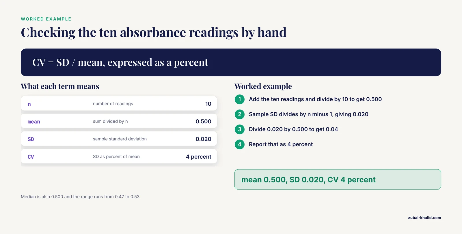
A small worked example anchors the rest of this guide. Suppose ten replicate absorbance readings from a plate reader are 0.48, 0.52, 0.51, 0.49, 0.50, 0.53, 0.47, 0.52, 0.50, and 0.48. Every tool on the market should return a mean of 0.500, a sample SD of 0.020, a coefficient of variation (CV, the SD divided by the mean, expressed as a percent) of 4 percent, a median of 0.500, and a range from 0.47 to 0.53. The IQR comes out at 0.035 under the most common percentile convention and 0.040 under another, a small difference worth remembering when you compare outputs across tools.
Descriptive Statistics Calculator for Lab Data Options at a Glance
Six tool families cover nearly every lab situation. The table compares them side by side, and the sections that follow explain each on its own terms.
| Option | Best for | Pros | Cons |
|---|---|---|---|
| Web calculator | One column, quick check | Free, instant, nothing to install | Manual entry errors, poor for wide tables, data leaves your machine |
| Spreadsheet (Excel, Google Sheets) | Routine datasets, teaching labs | Data, summaries, and charts in one file, reusable templates | Clicked steps are hard to replay, easy to grab the wrong range |
| Statistical package (SPSS, Prism, Minitab, JMP, SAS) | Report-driven and regulated work | Guided menus, formatted output, handles large files | License cost, menu steps leave no automatic record |
| Scriptable tools (R, Python) | Repeated analyses, pipelines, large data | Free, exact replay, automation | Coding skill required, slower first week |
| Bioinformatics platforms | Sequence and high-throughput data | Built for large biological datasets, saved histories | Overkill for a 12-row plate summary |
| Instrument or vendor software | Onboard analyzer summaries | Zero setup, native export parsing | Limited customization and data access, locked formats |
The Main Options for Lab Data, Explained
Web Calculators: Pros and Cons
Web-based descriptive statistics calculators take pasted or typed values and return the standard summary set in one click. Paste the ten absorbance readings from the example above into a typical web calculator and you get the mean 0.500 and the SD 0.020 within seconds, with nothing to install.
The pros are genuine for small jobs. These tools are free, they run in any browser, and they make honest second opinions, because recomputing a summary in an independent tool is one of the cheapest error checks available.
The cons decide most lab uses. Most web calculators accept one column at a time, so a 96-well plate or an analyzer export with dozens of columns becomes an afternoon of pasting. Entry is manual, which stacks transcription errors on top of whatever is already in the data. Results appear on screen and then vanish, leaving no record of which values produced them. Any values you paste also travel to someone else's server, which matters the moment a dataset holds patient identifiers, unpublished results, or material under a confidentiality agreement.
Use a web calculator for quick sanity checks and single-column summaries of non-confidential data. Treat it as a spot-check tool, not a system of record.
Spreadsheets: Pros and Cons
Spreadsheets are the default biology calculator in most labs because the raw values, the summaries, and the charts live in one file. Excel and Google Sheets both provide the descriptive set as functions: AVERAGE, MEDIAN, MIN, MAX, STDEV.S, VAR.S, QUARTILE, PERCENTILE, SKEW, and KURT. Excel's Analysis ToolPak add-in adds a one-click Descriptive Statistics report for a selected range. For the absorbance column, =STDEV.S(B2:B11) returns 0.020.
Two function choices trip people up. STDEV.S computes the sample SD by dividing by n minus 1, which is what lab data almost always calls for, because your replicates are a sample of the readings the assay could have produced. STDEV.P divides by n and describes a complete population. If a ten-reading summary should show an SD of 0.020 and the sheet shows 0.019, someone called STDEV.P.
The strengths go beyond arithmetic. A template built once, with summary cells wired to a paste area, becomes the lab's standard worksheet that every new dataset flows through. Sorting, filtering, and plotting happen in the same view, which is how most spread problems and outliers get caught by eye before any statistic is computed.
The cons are about process, not capability. Clicked steps leave no automatic record, so nobody can replay exactly how last month's summary was produced. Range selection is silent, and a formula dragged one row short changes an SD with no warning. Copy-paste from instruments can mangle dates, drop leading zeros from sample IDs, or split merged cells. Spreadsheets reward discipline: a locked template, one paste area, and summary formulas nobody edits by hand.
Menu-Driven Statistical Packages: Pros and Cons
Dedicated packages such as SPSS, GraphPad Prism, Minitab, JMP, and SAS sit between spreadsheets and code. Menus guide you toward sensible summaries, output arrives as formatted tables that drop into reports, and the software opens datasets far larger than a spreadsheet wants to handle.
Laboratory science leans on them. A randomized study of immunohematology training for laboratory sciences students, with 196 participants, analyzed questionnaire and practical exam results with descriptive and inferential statistics in SPSS version 26 [1]. A cytokine study measured serum interleukin-4 by ELISA (enzyme-linked immunosorbent assay) in brucellosis patients and sex- and age-matched controls, ran the analysis in SPSS version 21, and reported the group summaries in the mean ± SD format that remains the convention in biomedical writing, 1.42 ± 0.51 pg/mL in cases versus 1.31 ± 1.02 pg/mL in controls [2].
The pros follow from that track record. Guided dialogs reduce the odds of computing something meaningless, labeled output is easy to cite in a report, and the same software usually carries you into the inferential tests a project eventually demands.
The cons are cost and memory. Licenses are paid, often per seat, which matters for a teaching lab or a small startup. Menu-driven analysis is click history, not code, so when a reviewer asks exactly which cases were included, or when next month's export needs the same summary, you reconstruct the clicks from memory. Defaults can also shift between versions, so a colleague redoing your analysis in a different release may not match it exactly.
Scriptable Tools and the Bioinformatics Calculator
R and Python are free, open-source environments where a line or two of code produces the full summary set. In R, reading a file and summarizing every column takes two commands: readings <- read.csv("absorbance.csv") followed by summary(readings), which returns the minimum, first quartile, median, mean, third quartile, and maximum of each column at once. Dedicated functions such as sd(), IQR(), and quantile() fill in the rest. In Python, the pandas describe() method returns count, mean, standard deviation, minimum, maximum, and the quartiles of every column in one line.
The decisive advantage is that the script is the record. It states exactly which file was read, which rows were excluded, and which function ran in what order, so the same summary regenerates on new data without guesswork. That property scales from a ten-row teaching dataset to pipelines that summarize instrument exports every night.
Non-statisticians do learn this. In one teaching case study, instructors piloted R with nine non-statisticians as a complement to SPSS in a multivariate course for healthcare graduate students, then extended the approach to community stakeholders with no statistics background [3]. The first week with code is slower than a spreadsheet, and every week after that is faster.
For sequence data, genomics, and other high-throughput work, the bioinformatics calculator is usually a workflow platform or a notebook rather than a single web page. Platforms built for biological data chain summary steps into larger analyses, save a history of every operation, and rerun the whole chain when new data arrive. Notebooks in Jupyter or R Markdown interleave code, summaries, and interpretation in one shareable document that reruns end to end.
The cons are the learning curve and overbuilding. A script that summarizes one column for one report is overkill, and a disorganized script folder can end up as unreproducible as a pile of clicks.
Instrument and Vendor Software: Pros and Cons
Analyzers, plate readers, and sequencers ship with onboard summary functions, and most vendors sell companion software for post-run statistics. The pros are real: zero setup, native parsing of the instrument's own export format, and summaries that appear the moment a run ends.
The cons come from the vendor relationship. Output formats are locked, customization is limited, and pulling raw values out for independent analysis depends on export steps the vendor controls. An evaluation of a five-year digital health implementation project across California counties found that vendors supplemented internal expertise but offered limited customization and data access [4], and laboratory software contracts often follow the same pattern. Treat vendor summaries as a first look, then move the numbers into a tool you control before anything enters a report.
The Criteria That Decide Real Choices
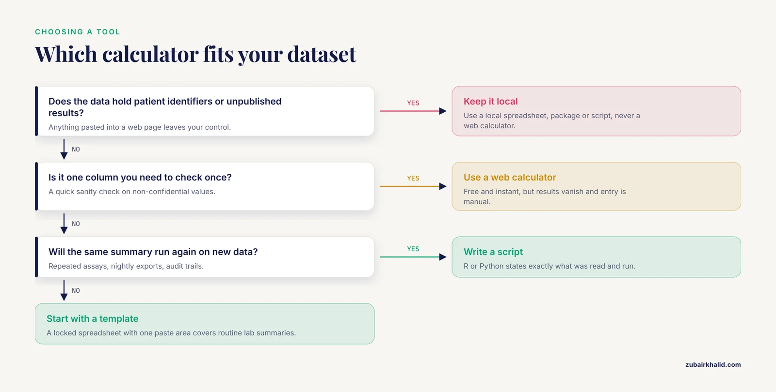
Compare candidate tools on seven criteria, roughly in this order.
- Dataset size and shape. A web calculator handles one column. A spreadsheet handles hundreds of rows comfortably and thousands with care. Packages and scripts handle the wide tables that analyzers, sequencers, and imaging systems export.
- Reproducibility. Ask whether the analysis will run again with new data. If yes, scripts win, spreadsheet templates come second, and one-off menu clicks come last. A useful test is to hand the file and the instructions to a colleague and see whether they can regenerate your summary without asking you a question.
- Confidentiality. Anything uploaded to a web calculator or a cloud sheet leaves your control. Local installs keep values on the machine.
- Statistical depth. Projects rarely stay descriptive. A linked-data study in Wales planned descriptive and inferential statistics, along with propensity score matching (a method for building comparable groups from non-randomized data), on census-level adult care records from the outset [5]. If inferential work is plausible, choose a tool that carries you there without a migration.
- Reporting conventions. Biomedical reports expect mean ± SD for symmetric data and median with IQR for skewed data, always with n and units. Packages produce that formatting by default, spreadsheets need a template, and web calculators hand you raw numbers to format yourself.
- Team skills and turnover. A tool nobody else in the lab can open is a liability. Weigh who maintains the template or script after you rotate off the project.
- Vendor terms. Before building on a vendor platform, read exactly what you can export and customize, and what happens to data stored there.
Worked Scenarios
Scenario 1: A teaching lab report
Three treatment groups, ten readings each, one afternoon to write it up. A spreadsheet template is the right tool. Paste each group into its own column, compute AVERAGE and STDEV.S beneath, report each group as mean ± SD, and plot the three means with error bars in the same sheet. The whole analysis survives as one file a grader or collaborator can open. If the course later asks for a t test, the same file moves into a package without re-entry.
Scenario 2: An analyzer export with dozens of parameters
Modern hematology and flow cytometry platforms export wide tables. A dengue study at a blood disease institute in Karachi shows the shape of the problem: 389 febrile patients were screened, complete blood counts ran on Sysmex XN analyzers, and all 65 cell population data (CPD) parameters, the analyzer-derived measures of white cell characteristics beyond the standard count, went through descriptive analysis in SPSS version 25 before receiver operating characteristic curves, which plot sensitivity against specificity across candidate cutoffs, were used to evaluate cutoff values [6]. A web calculator cannot hold that table. A spreadsheet can, but once per-parameter summaries and correlations multiply, a package or a script is the better fit.
Scenario 3: Transferring reference intervals between populations
Reference intervals, the ranges that define usual results in healthy people, are a descriptive-statistics product. One study built two real-world datasets of 10,000 free thyroxine results each, one from the US and one from Europe, and compared descriptive statistics, density plots, and cumulative distributions between them [7]. Percentile differences were estimated by case resampling bootstrapping, which redraws the data with replacement to gauge how stable an estimate is, then checked against an acceptance criterion of 7.8 percent or less tied to inter-individual biological variability. The means came out at 16.1 pmol/L in the US and 16.4 pmol/L in Europe, with medians of 15.4 and 15.8 pmol/L. This is script territory: quantile functions, resampling, and acceptance rules are awkward in menus and impossible in a one-column web calculator.
Scenario 4: Comparing results across laboratories
When several labs run the same assay, descriptive statistics are the shared language for asking whether the labs agree. In a multi-laboratory drug safety study, five laboratories tested 28 drugs with manual patch clamp, a technique that measures currents through individual ion channels, at hERG, the cardiac potassium channel whose block is the most common mechanism underlying drug-induced QTc prolongation [8]. Results were characterized with descriptive statistics and meta-analysis (pooled analysis across studies). Systematic differences in block potencies appeared for one laboratory across the first 21 drugs and disappeared for the last seven, retests mostly agreed within 1.6-fold, and one laboratory's retest of a single drug differed 7.6-fold from its own first result. Per-lab, per-drug summaries on this scale are exactly the job a reproducible tool should turn out on schedule.
Common Mix-Ups
- SD versus standard error. The standard error of the mean is the SD divided by the square root of n, so it shrinks as n grows. The SD does not. Reporting the standard error where readers expect the SD makes noisy data look tight.
- Mean with SD for skewed data. When the SD approaches the mean, as in the interleukin-4 control group above, the distribution is often skewed, and the median with IQR describes the center more honestly. Compute both, then report what fits.
- Sample versus population SD. Lab replicates are samples, so the n minus 1 version (STDEV.S) is the default.
- Replicates versus independent experiments. Ten readings from one plate are not ten independent experiments. State which n you are summarizing.
- Below-limit values as zeros. Results below a detection limit are censored observations, not true zeros, and averaging them as zeros biases every summary downward.
- Rounding too early. Round for display, not for intermediate steps, or downstream calculations inherit the error.
- Percentile conventions. Quartiles can differ slightly between tools because software uses different percentile methods, which is why the absorbance example's IQR is 0.035 under one convention and 0.040 under another.
Common Mistakes and Limitations
Summarizing before checking quality control. Quality control (QC) samples are known specimens run alongside unknowns to verify that an assay behaved during the run. Guidance developed for environmental exposure measurements urges researchers to examine laboratory and field QC data closely before interpreting chemical measurements, and observes that many studies do not adequately describe or interpret QC assessments, partly because the guidance is fragmented and hard to find [9]. A calculator will happily summarize a run that the QC disqualifies. Check QC first, summarize second.
Assuming the tool catches design errors. A descriptive statistics calculator computes what you give it. It will not flag a swapped control column, a unit change between runs, or a plate read twice.
Pooling before characterizing between-lab variability. The multicenter hERG scenario above shows that even standardized protocols leave lab-to-lab differences that deserve their own summaries. Build per-lab summaries into any comparison instead of pooling everything blindly.
Letting metadata drift. Lab values without context cannot be reused. Work in nanosafety responded to this problem by merging existing standards into a minimum information table with six modules, covering general and material information among others, so that datasets carry the details needed for reuse [10]. Whatever tool you choose, record instrument, units, lot numbers, and dates alongside the numbers, in the same file or a linked data dictionary.
Trusting defaults blindly. Default SD type, default percentile method, and default handling of missing values vary between tools. Learn your tool's defaults before its output goes into a report.
The standing limitation is that no calculator replaces judgment about your own dataset. Decisions that affect patient care, regulatory submissions, or publication claims deserve review by a qualified laboratory professional or statistician.
Frequently Asked Questions
What is the best descriptive statistics calculator for lab data?
There is no single best tool, because the right choice depends on dataset size, confidentiality, and whether the analysis will be repeated. For most lab work, a spreadsheet template covers daily summaries, a menu-driven package such as SPSS covers report-driven projects, and scripts in R or Python cover anything that must be replayed exactly.
Can I use Excel as a biology calculator for lab statistics?
Yes. Excel computes the full descriptive set through functions such as AVERAGE, MEDIAN, and STDEV.S, plus a Descriptive Statistics report in the Analysis ToolPak add-in. Use STDEV.S for sample data, lock your summary cells, and keep one paste area to avoid silent range errors.
What is the difference between descriptive and inferential statistics?
Descriptive statistics summarize the dataset you have, using numbers such as the mean, median, SD, and IQR. Inferential statistics use the same data to test hypotheses or estimate confidence intervals about a larger population. Most lab projects need the descriptive layer first.
When should I move from a calculator to R or Python?
Move when the analysis repeats, the datasets grow beyond what a spreadsheet opens comfortably, or someone needs an exact record of every step. Scripts regenerate the same summary on new data with no guesswork.
Are online descriptive statistics calculators safe for confidential lab data?
Treat anything pasted into a web calculator as data that has left your control. For patient identifiers, unpublished results, or contract-covered material, use a local spreadsheet, package, or script instead.
Which numbers should I report from lab data?
Report n, the mean with SD for symmetric data, or the median with IQR for skewed data, always with units. Add the range or percentiles when the extremes matter, and state whether n counts replicates or independent experiments.
Sources
- Blended learning in laboratory science education: comparison of flipped classroom and traditional lectures in immunohematology training.
- Comparison of the serum level of interleukin-4 in patients with brucellosis and healthy controls.
- Teaching Confirmatory Factor Analysis to Non-Statisticians: A Case Study for Estimating Composite Reliability of Psychometric Instruments.
- Implementing digital mental health tools in the public behavioral health systems: a multi-city/county evaluation of California's Help@Hand project.
- Understanding Inequalities in Adult Social Care in Wales: Protocol for the CARE Lab Linked Administrative Data Study.
- Cell Population Data Parameters in Dengue-Is There Any Significance? A Single-Center Study.
- Feasibility of using real-world free thyroxine data from the US and Europe to enable fast and efficient transfer of reference intervals from one population to another.
- Multi-laboratory comparisons of manual patch clamp hERG data generated using standardized protocols and following ICH S7B Q&A 2.1 best practices.
- Wrangling environmental exposure data: guidance for getting the best information from your laboratory measurements.
- Digital research data: from analysis of existing standards to a scientific foundation for a modular metadata schema in nanosafety.