Ceiling Effect in Statistics: Definition and Examples

By Dr. Zubair Khalid, DVM, MS, PhD · 2026-10-03

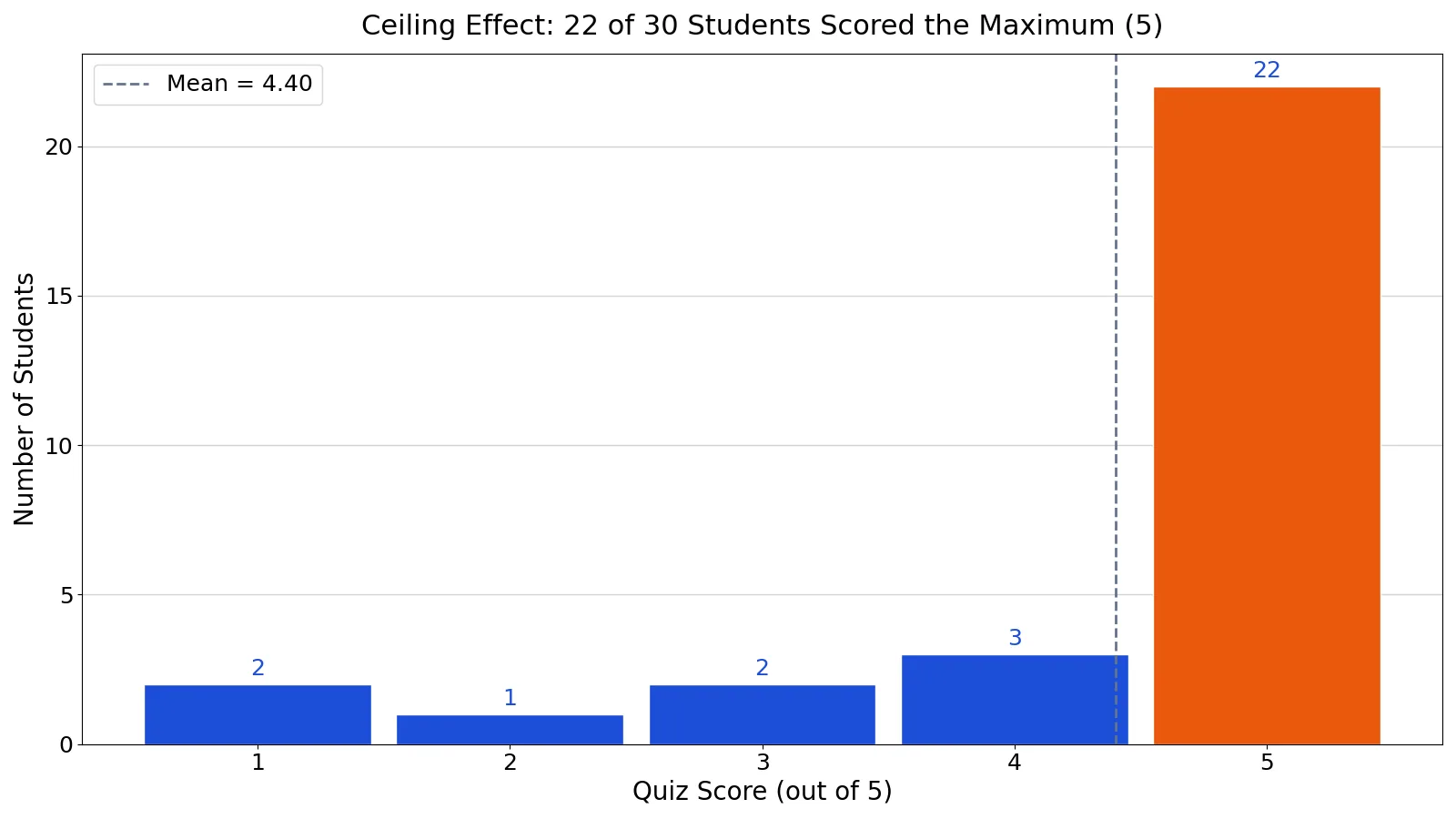
A ceiling effect in statistics occurs when a large share of scores pile up at the highest possible value on a scale. Once respondents hit that top value, the instrument cannot record how much better they really are, so the data lose the ability to distinguish them. This matters because ceiling effects statistics produce can bias means, shrink variance, and hide real treatment effects.

Quick Answer

A ceiling effect is a scale attenuation problem: scores cluster at the upper limit of a measure [1].
It appears when a task is too easy, a scale has too few response options, or a treatment stops producing gains above a certain level [1][2].
The damage is loss of variance. If most people score the maximum, the measure cannot separate them [2].
In longitudinal studies the problem worsens over time, because more participants reach the ceiling at later waves [3].
In trials, a ceiling effect can make an active drug look no better than placebo, which fails the trial [4].

What the Ceiling Effect Means

In plain terms, a ceiling effect is what happens when a test or survey runs out of room at the top. Everyone who could score high does score high, and the numbers stop reflecting real differences between people.

The precise statistical definition is narrower. The ceiling effect is one of two scale attenuation effects, the other being the floor effect [1]. It is observed when an independent variable no longer has an effect on a dependent variable, or when there is a level above which variance in a variable is no longer measurable [1]. In social science survey work, the term describes data where the majority of responses sit close to the upper limit of the response scale [2].

Two settings use the phrase. In pharmacology, a ceiling effect means a drug produces no further benefit above a certain dose [1]. In data gathering, it means the instrument's highest category caps what can be recorded, such as a survey that groups all high earners into one income bracket [1].

How It Works

There is no single formula for a ceiling effect, but you can quantify it directly. The ceiling proportion is the share of observations sitting at the maximum:

$$P_{\text{ceiling}} = \frac{n_{\text{max}}}{n}$$

where $n_{\text{max}}$ is the count of cases at the highest possible score and $n$ is the total number of cases. A high value of $P_{\text{ceiling}}$ signals that the measure is compressed at the top.

The mechanism behind the distortion is variance loss. Variance is the average squared deviation from the mean:

$$s^2 = \frac{\sum_{i=1}^{n}(x_i - \bar{x})^2}{n-1}$$

When many $x_i$ equal the maximum, those deviations shrink toward zero, so $s^2$ falls. A smaller denominator in effect size formulas such as Cohen's $d$ then inflates the standardized difference, while the true difference between groups may be understated because the top group cannot score higher. The measure is censored, meaning values above the ceiling exist in reality but are recorded as the ceiling value.

Worked Example

A class of 30 students takes a quiz scored from 1 to 5. The instructor wants to know how well the class performed and whether the quiz separates strong students from weak ones.

student_id	score	student_id	score	student_id	score
1	5	11	5	21	5
2	5	12	5	22	5
3	5	13	5	23	4
4	5	14	5	24	4
5	5	15	5	25	4
6	5	16	5	26	3
7	5	17	5	27	3
8	5	18	5	28	2
9	5	19	5	29	1
10	5	20	5	30	1

The full score list is [5, 5, 5, 5, 5, 5, 5, 5, 5, 5, 5, 5, 5, 5, 5, 5, 5, 5, 5, 5, 5, 5, 4, 4, 4, 3, 3, 2, 1, 1].

Step by step:

Number of students: $n = 30$
Sum of scores: 132, so the mean is $132/30 = 4.4000$
Median: 5.0000
Mode: 5
Sample standard deviation ($n-1$): 1.1919
Population standard deviation: 1.1719
Sample variance: 1.4207
Q1 (PERCENTILE.INC): 4.2500
Q3 (PERCENTILE.INC): 5.0000
IQR: $5.0000 - 4.2500 = 0.7500$
Students at the ceiling (score = 5): 22
Ceiling percentage: $22/30 = 73.3333\%$
Range: $5 - 1 = 4$

The same values come out of a spreadsheet. =AVERAGE(A2:A31) returns 4.4000, =STDEV.S(A2:A31) returns 1.1919, =QUARTILE.INC(A2:A31,1) returns 4.2500, =QUARTILE.INC(A2:A31,3) returns 5.0000, and =COUNTIF(A2:A31,5) returns 22.

import statistics
scores = [5, 5, 5, 5, 5, 5, 5, 5, 5, 5, 5, 5, 5, 5, 5, 5, 5, 5, 5, 5, 5, 5, 4, 4, 4, 3, 3, 2, 1, 1]
mean = statistics.mean(scores)          # 4.4000
sd_s = statistics.stdev(scores)         # 1.1919
ceiling = sum(1 for s in scores if s == 5)  # 22
pct = 100 * ceiling / len(scores)       # 73.3333

Output: mean=4.4000, sample_sd=1.1919, ceiling_count=22, ceiling_pct=73.3333%

The histogram shows a tall spike at score 5, where 22 students (73.3%) sit at the maximum. Mean = 4.40, sample SD = 1.19.

How to Interpret It

Read the ceiling percentage first. Here, 73.3% of students scored the maximum, so the quiz cannot tell you which of those 22 students learned more. The mean of 4.40 looks strong, but it is a compressed summary of a measure that ran out of range.

Notice how the median and mode both equal 5 while the mean is 4.40. That gap is a classic signature of a ceiling effect. The mean is dragged down by the few low scores, while the median sits at the ceiling. If you only reported the mean, you would miss that most of the class is indistinguishable at the top. This is one reason to compare the mean and median together when you check a distribution.

The IQR of 0.75 is also telling. The middle half of the class spans less than one score point, so the measure has almost no resolution where most of the data live. Low variability at the top is the core problem, and it feeds directly into effect size estimates and any test that assumes spread in the data.

When to Use It (and when not to)

You do not "use" a ceiling effect. You detect it and respond to it. Check for it whenever you analyze test scores, satisfaction ratings, symptom scales, or any bounded instrument, especially in longitudinal designs where participants improve across waves [3].

When you find one, you have options. Choose a previously validated measure with a wider range, run a pilot test before the main study, or combine instruments to capture the top of the distribution [1]. For longitudinal data, a Tobit growth curve model handles censored values well, while an ordinary growth curve model can pick the wrong model and bias the estimated shape of change [3].

Do not treat a ceiling effect as proof that a program worked. High scores can mean the task was too easy, not that learning was strong. And do not apply ceiling corrections when the pile-up is genuine. If a safety training really does produce near-universal mastery, the ceiling reflects reality, and the right fix is a harder follow-up measure, not a statistical adjustment.

Ceiling Effect vs Floor Effect

The floor effect is the mirror image: scores cluster at the bottom of the scale instead of the top. Both are scale attenuation effects, and both destroy variance [1]. The difference is where the compression happens and what it implies about your sample.

Feature	Ceiling effect	Floor effect
Where scores pile up	Top of the scale	Bottom of the scale
Typical cause	Task too easy, scale too narrow	Task too hard, scale too narrow
Effect on mean	Pulled toward the maximum	Pulled toward the minimum
Effect on variance	Shrinks at the top	Shrinks at the bottom
Common setting	Mastery tests, satisfaction surveys	Hard tests, severe symptom scales
Trial consequence	Active drug looks like placebo [4]	Active drug looks like placebo [4]

Common Mistakes

Reporting only the mean. A mean of 4.40 hides that 73.3% of scores are identical. Always report the ceiling percentage and the median alongside the mean.
Assuming high scores mean high performance. A ceiling effect often means the test was too easy. Check item difficulty before praising the results.
Ignoring the ceiling in longitudinal work. More participants hit the ceiling at later waves, which biases the estimated growth curve [3]. Model the censoring explicitly.
Using a scale with too few points. A 1 to 5 scale caps quickly. Wider scales give high performers room to separate.
Skipping pilot testing. A small pilot reveals the ceiling before you commit to a full study, when adjustments are still cheap [1].
Misreading a failed trial. If an active control performs no better than placebo, a ceiling effect may be the cause, and the trial cannot establish assay sensitivity [4].

Limitations

A ceiling effect is a property of your measurement, not a flaw you can always fix after the fact. Once data are collected at the ceiling, the true values above it are gone. You cannot recover the differences between the 22 students who all scored 5, because the instrument never recorded them. Statistical corrections such as Tobit models help with censored data, but they rely on assumptions about the unobserved distribution and will not rescue a measure that was simply too easy [3].

Detection is also judgment-based. There is no universal cutoff for how much pile-up counts as a ceiling effect. A 20% ceiling proportion may be harmless in one study and damaging in another, depending on the analysis. Report the ceiling percentage, the median, and the variance so readers can judge for themselves, and treat any strong claim about group differences with caution when the top of the scale is crowded.

Frequently Asked Questions

What is a ceiling effect in simple terms?

It is when most scores hit the highest possible value on a test or survey, so the measure can no longer tell high scorers apart. The data look strong on average but carry little information at the top.

How do you detect a ceiling effect?

Compare the mean, median, and mode, and compute the share of cases at the maximum. In the quiz example, the median and mode are both 5 while the mean is 4.40, and 73.3% of students scored the maximum. A large gap between mean and median plus a high ceiling percentage is a clear signal.

Does a ceiling effect bias results?

Yes. It shrinks variance at the top, which distorts effect sizes and can hide real differences between groups. In longitudinal studies it leads to incorrect model selection and biased estimates of the shape of change [3]. In trials it can make an active treatment look no better than placebo [4].

How is a ceiling effect different from a floor effect?

A ceiling effect compresses scores at the top of the scale, and a floor effect compresses them at the bottom. Both are scale attenuation effects that reduce variance, but they point to opposite problems: a task that is too easy versus one that is too hard [1].

How can you prevent a ceiling effect?

Choose a previously validated measure with a wide enough range, run a pilot test before the main study, or combine instruments to capture the top of the distribution [1]. If the pile-up is genuine, switch to a harder or more sensitive measure instead of adjusting the statistics.