Essential Calculator Functions for Molecular Biology Labs
By Dr. Zubair Khalid, DVM, MS, PhD ·
By the end of this guide, you will be able to run every routine calculation a molecular biology bench asks for: turning an absorbance reading into a DNA concentration, counting the molecules in a stock tube, planning dilutions, scoring primers, setting up a ligation, sizing gel bands, and converting qPCR Ct values into fold changes. You need three things on hand: a scientific calculator or a spreadsheet, a free sequence tool such as GENtle, and your own data, whether that is an A260 reading, a primer sequence, a photo of a DNA ladder, or a table of Ct values.
These are the essential calculator functions for molecular biology lab work. None of them requires paid software, and all of them reduce to a handful of formulas you can memorize once, paste into a spreadsheet, and reuse for years.
Why Molecular Biology Labs Run on Calculations
Every wet lab technique produces a number that means nothing on its own. A spectrophotometer prints an absorbance, not a usable concentration. A gel camera records band positions, not base pair counts. A qPCR instrument reports cycles, not fold changes. The conversion between raw instrument output and a number you can put in a notebook is the job of the calculator.
This pairing of computation and bench work is now standard training. A molecular genetics laboratory course built around original research has students apply bioinformatics and cell biology side by side, moving between sequence data and wet lab experiments within a single course [1]. An introductory molecular biology course takes this further with a six-week project in which students identify an unknown protein using open access databases and then use the recovered genomic DNA sequence to design primers and amplify the corresponding gene from dissected Drosophila tissue [2]. That path from database to pipette runs through arithmetic at every step, and curricula increasingly add skills-based laboratory components precisely to build this quantitative fluency [3].
The practical takeaway is simple. If you can run the calculations in this article without hesitation, you can move between the computational and technical halves of almost any molecular project without stalling.
Your Toolkit: From Handheld Biology Calculator to Bioinformatics Calculator
Most lab math lives at one of three tiers.
Tier 1, the scientific calculator. The functions that matter are log10, 10^x, scientific notation entry (the EE or EXP key), parentheses, and memory storage. Nearly every formula in this guide uses powers of ten, so find the EE key on your model before your first calculation, not during it.
Tier 2, the spreadsheet. A spreadsheet beats a handheld calculator for anything you will repeat, because the formula stays saved and recalculates when inputs change. Two error messages you will eventually see are #VALUE!, which means a cell your formula references contains text instead of a number, and #DIV/0!, which means the formula divided by zero, usually because a length or concentration cell was left empty. Fix both by checking the referenced cells, not the formula.
Tier 3, the dedicated bioinformatics calculator. Sequence work outgrows spreadsheets quickly. GENtle is a free multi-purpose molecular biology tool that handles sequence viewing, annotation, restriction analysis, and primer design in one program [4]. For complex engineering projects, the Molecular Cloning Designer Simulator (MCDS) goes further: it is an all-in-one cloning design, simulation, and management platform with an interactive flow-chart interface that can execute a user-defined workflow of cloning steps in a single run and store results and comments for the whole project [5]. These tools do not replace the formulas below. They automate them, and you still need the arithmetic to catch a wrong input.
Key Formulas at a Glance
| Function | Formula | Inputs you need | Common trap |
|---|---|---|---|
| dsDNA concentration | ng/µL = A260 × 50 × dilution factor | A260, dilution factor | Using 50 for RNA |
| Purity check | A260 ÷ A280, A260 ÷ A230 | Both absorbances | Judging purity from one ratio |
| Copy number | copies = (mass in g × 6.022 × 10^23) ÷ (bp × 660) | Mass, length in bp | Mixing ng and µg |
| Dilution | C1V1 = C2V2 | Stock and target concentration, final volume | Dropping the dilution factor |
| GC content | (G + C) ÷ total bases × 100 | Primer sequence | Counting ambiguous bases |
| Wallace Tm | 2 × (A + T) + 4 × (G + C) | Primer sequence | Applying it to long probes |
| Insert mass for ligation | ng insert = ng vector × (insert bp ÷ vector bp) × ratio | Masses, lengths, molar ratio | Treating the ratio as mass-based |
| Gel band size | Linear fit of log10(bp) vs distance | Ladder bands, band distance | Extrapolating past the ladder |
| qPCR fold change | 2^(-ΔΔCt) | Four Ct values | Assuming perfect efficiency |
| Protein size | kDa ≈ amino acids × 110 ÷ 1000 | ORF length in bp | Forgetting the stop codon |
Calculator Functions for Molecular Biology Lab, Step by Step
The seven walkthroughs below cover the calculations you will reach for weekly. Each one gives the formula, a worked example, a way to check the result, and the error most likely to bite you.
Step 1: Nucleic Acid Concentration from Absorbance
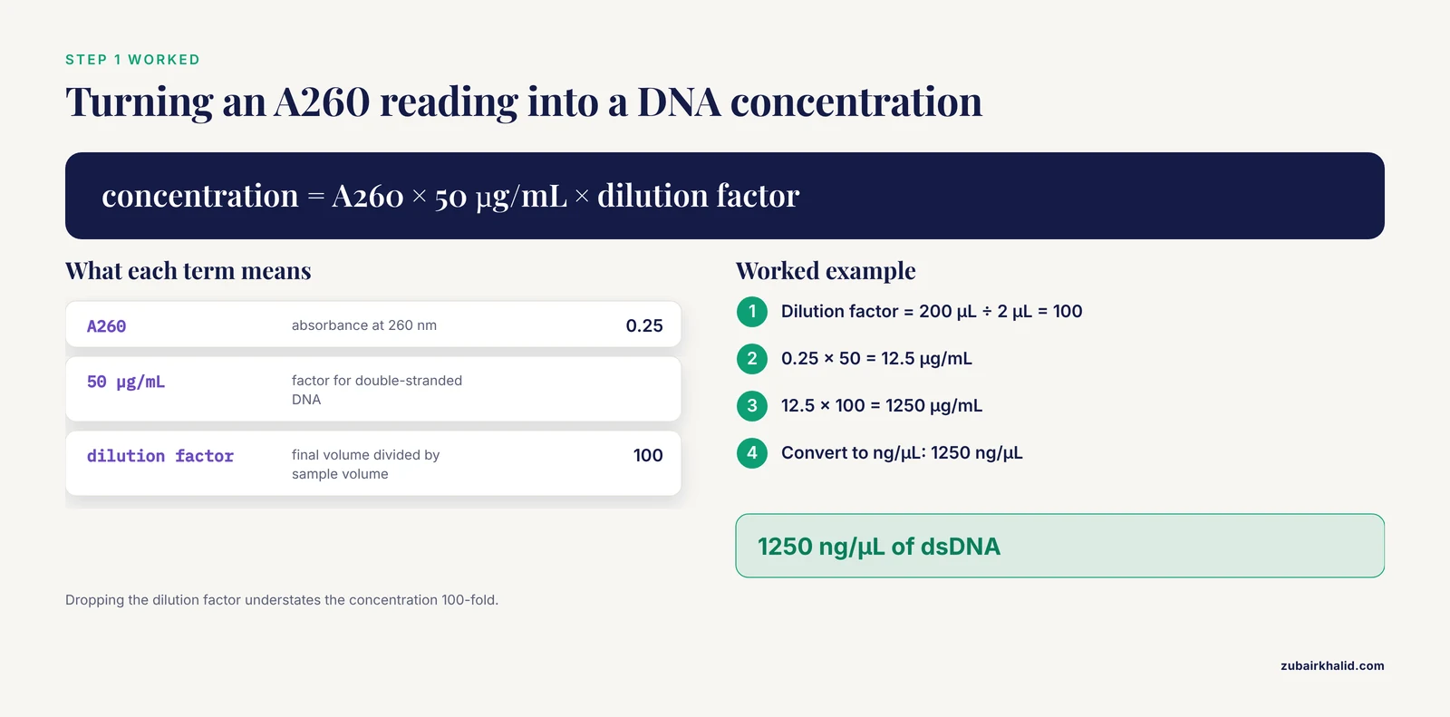
A spectrophotometer reports absorbance at 260 nm, written A260, the wavelength where nucleic acids absorb most strongly. The Beer-Lambert law (A = ε × l × c) connects absorbance to concentration, and for a standard 1 cm path length the conversion factors are standard values used across molecular lab manuals: one A260 unit equals 50 µg/mL double-stranded DNA, 33 µg/mL single-stranded DNA, or 40 µg/mL RNA.
Worked example. You dilute 2 µL of a plasmid prep into 198 µL of water and read A260 = 0.25. The dilution factor is 200 ÷ 2 = 100.
concentration = A260 × 50 µg/mL × dilution factor
              = 0.25 × 50 × 100
              = 1250 µg/mL
              = 1250 ng/µL
Read purity from the same scan. A260/A280 near 1.8 suggests reasonably clean DNA, near 2.0 suggests clean RNA, and A260/A230 near 2.0 indicates low carryover of salts, phenol, or protein.
Check the result by reading a second independent dilution. The two values should agree closely. The most common error is forgetting the dilution factor, which understates the concentration by the full factor, here 100-fold.
Step 2: Copy Number of a DNA Stock
Copy number tells you how many molecules are in the tube, which you need for qPCR standards, transformation calculations, and ligation planning. The formula uses Avogadro's number (6.022 × 10^23 molecules per mole) and the average mass of one base pair of double-stranded DNA, 660 g/mol.
AVOGADRO = 6.022e23
BP_MASS = 660  # grams per mole per base pair

def copy_number(mass_ng, length_bp):
    mass_g = mass_ng * 1e-9
    return (mass_g * AVOGADRO) / (length_bp * BP_MASS)

print(copy_number(10, 5000))
Expected output:
1824848484.8484848So 10 ng of a 5000 bp plasmid contains about 1.8 × 10^9 molecules. A useful anchor for checking any copy number result: 1 pmol of a 1000 bp DNA fragment weighs 0.66 µg, because 1000 bp × 660 g/mol = 6.6 × 10^5 g/mol. If your answer implies a pmol value wildly inconsistent with that anchor, recheck the units. The classic mistake here is entering mass in ng while treating it as grams, which throws the answer off by 10^9.
Step 3: Dilutions and Serial Dilutions
The dilution equation C1V1 = C2V2 covers nearly every dilution you will make, where C1 and V1 are the stock concentration and the volume you take, and C2 and V2 are the target concentration and final volume.
Worked example. You have a 100 µM primer stock and need 500 µL of a 50 µM working solution.
V1 = (C2 × V2) ÷ C1
   = (50 µM × 500 µL) ÷ 100 µM
   = 250 µL stock + 250 µL water
For a serial dilution, the same equation applies repeatedly. A 1:10 series made by transferring 100 µL into 900 µL fresh diluent at each step gives a cumulative dilution factor of 10 per step, so tube 4 is 1:10,000 relative to the original. Label each tube with both the concentration and the cumulative dilution factor, because you will need the factor later for qPCR standard curves.
Check the result by working backward: the concentration times the cumulative dilution factor must return the original stock concentration. The common error is adding the transfer volume to a final volume that already includes it, which silently changes every downstream factor.
Step 4: Primer Statistics: GC Content and Melting Temperature
Melting temperature (Tm) is the temperature at which half of the primer-template duplexes separate, and it predicts where to set your annealing temperature. GC content is the fraction of guanine and cytosine bases, which stabilize the duplex.
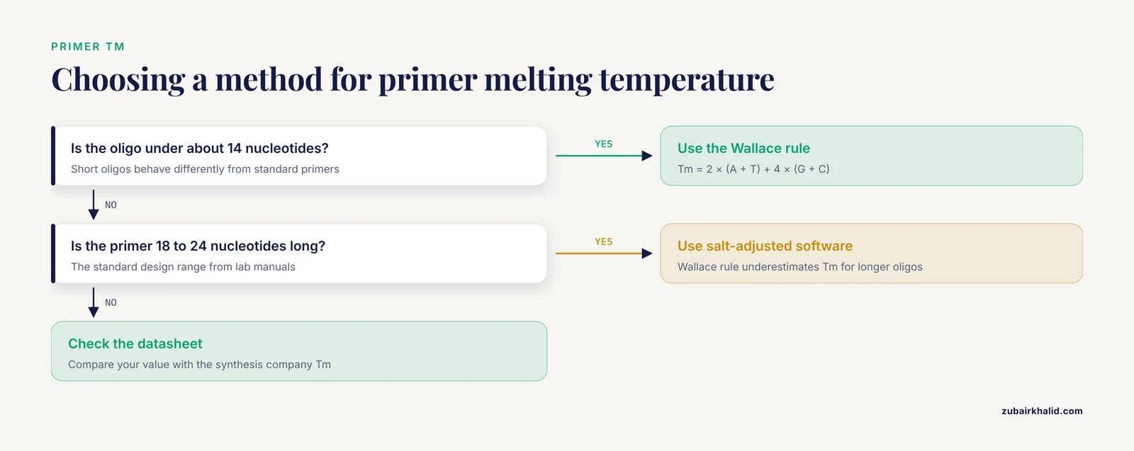
For short oligonucleotides, roughly under 14 nucleotides, the Wallace rule gives a quick estimate:
Tm = 2 × (A + T) + 4 × (G + C)For standard 18 to 24 nucleotide primers, use a salt-adjusted or nearest-neighbor calculation in sequence software instead, because the Wallace rule underestimates Tm for longer oligos.
def gc_percent(seq):
    seq = seq.upper()
    gc = sum(seq.count(base) for base in "GC")
    return 100 * gc / len(seq)

def wallace_tm(seq):
    seq = seq.upper()
    gc = sum(seq.count(base) for base in "GC")
    at = len(seq) - gc
    return 2 * at + 4 * gc

primer = "ATGGCCTAGGTCAATGCTGA"
print(gc_percent(primer), wallace_tm(primer))
Expected output:
50.0 60Standard design targets from lab manuals: primers 18 to 24 nucleotides long, GC content between 40 and 60 percent, both primers of a pair within a few degrees of Tm, and an annealing temperature set 3 to 5 °C below the lower primer Tm. This is exactly the arithmetic students perform when they move from a genomic DNA sequence to working primers, as in the Drosophila project described earlier [2].
Check your hand calculation against the Tm printed on the oligo datasheet from the synthesis company. A large discrepancy usually means you used the Wallace rule on a long primer.
Step 5: Ligation Setup: How Much Insert per Vector
Ligation recipes are specified as molar ratios, meaning ratios of molecule counts, not masses. Because a short insert weighs less per molecule than a long vector, you must convert. A 3:1 insert-to-vector molar ratio is the standard starting point.
ng insert = ng vector × (insert bp ÷ vector bp) × desired ratioWorked example. You have 50 ng of a 3000 bp vector and a 750 bp insert at 3:1.
ng insert = 50 × (750 ÷ 3000) × 3 = 37.5 ngCheck the result by asking whether the numbers make physical sense: the insert is one quarter the length of the vector, so one quarter of the vector mass gives an equal molecule count, and the 3:1 ratio triples that. Software helps here as designs grow. MCDS was built precisely to simulate multi-step cloning and recombineering workflows and to store the design details, so the arithmetic gets checked before reagents are committed [5].
Always set up a vector-only control to measure background from uncut or re-ligated vector. The calculator predicts the ideal assembly, and the control tells you what actually happened.
Step 6: Estimating DNA Fragment Sizes from a Gel
DNA fragments migrate through agarose at a rate inversely related to the logarithm of their length, so fragment size and migration distance follow a straight line when distance is plotted against log10(bp). To size an unknown band, fit a line through nearby ladder bands and interpolate.
import math

ladder = {1000: 20.0, 500: 28.0}  # bp: distance in mm

def size_at(distance_mm, ladder):
    (bp1, d1), (bp2, d2) = ladder.items()
    slope = (math.log10(bp2) - math.log10(bp1)) / (d2 - d1)
    return 10 ** (math.log10(bp1) + slope * (distance_mm - d1))

print(round(size_at(24.0, ladder)))
Expected output:
707A band 24 mm from the well, between a 1000 bp ladder band at 20 mm and a 500 bp band at 28 mm, is about 707 bp. Students working through a virtual gel electrophoresis module worked out exactly this relationship between fragment size and migration distance and then evaluated their band interpretations against electrophoresis theory [6].
Check the result by confirming the unknown band falls between the two ladder bands you used. Extrapolating outside them is unreliable. Measure every distance from the same reference point, usually the well front, and use the ladder from the same gel, because agarose concentration and buffer change the curve.
Step 7: qPCR Fold Change with ΔΔCt
Quantitative PCR reports Ct, the amplification cycle at which fluorescence crosses a detection threshold, which is proportional to the logarithm of the starting template quantity. The ΔΔCt method converts four Ct values into a fold change.
The steps:
- ΔCt(treated) = Ct(target, treated) - Ct(reference, treated)
- ΔCt(control) = Ct(target, control) - Ct(reference, control)
- ΔΔCt = ΔCt(treated) - ΔCt(control)
- Fold change = 2^(-ΔΔCt)
The reference gene is a housekeeping gene whose expression should not change between conditions. Worked example: treated target Ct 22, treated reference Ct 18, control target Ct 20, control reference Ct 18. Then ΔCt(treated) = 4, ΔCt(control) = 2, ΔΔCt = 2, and the fold change is 2^(-2) = 0.25, a fourfold decrease.
def fold_change(ct_target_treated, ct_ref_treated,
                ct_target_control, ct_ref_control):
    d_treated = ct_target_treated - ct_ref_treated
    d_control = ct_target_control - ct_ref_control
    dd = d_treated - d_control
    return 2 ** (-dd)

print(fold_change(22, 18, 20, 18))
Expected output:
0.25This arithmetic applies across target types. RT-qPCR is a standard wet lab technique for detecting and quantifying circular RNAs, and the same ΔCt pipeline handles those assays [7]. The key assumption is that the amplification efficiency is close to 100 percent. Verify efficiency with a dilution series before reporting exact fold values, because the 2^(-ΔΔCt) formula degrades quickly at lower efficiency.
From Bench Arithmetic to Bigger Models
The same sequence arithmetic scales up to protein-level questions. An open reading frame (ORF) of 981 bp encodes 981 ÷ 3 = 327 codons, or 326 amino acids after removing the stop codon. At an average residue mass of about 110 Da, the predicted protein is roughly 35.9 kDa. Teaching modules that mutate a protein in silico and connect the predicted structural changes to in vivo and in vitro analyses build directly on this sequence-to-protein arithmetic [8].
Beyond single calculations, molecular biology increasingly runs on formal mathematical models. Work on chromatin in fission yeast aims to establish physical and mathematical models of chromatin fiber architecture, connecting molecular-scale data to higher-order structure [9]. At the data-analysis end, transcriptome and metabolome measurements from individual plants have been used to quantitatively predict phenotypes and gene function, showing how the numbers generated at the bench feed predictive models in the field [10]. The calculator skills in this article are the foundation those larger analyses stand on.
How to Check Your Work
Four habits catch most calculation errors before they cost reagents.
- Run an order-of-magnitude sanity check. Know your anchors: 1 pmol of 1000 bp DNA weighs 0.66 µg, and 1 A260 unit of dsDNA is 50 µg/mL.
- Compute anything high-stakes twice, once by hand and once in software. Agreement between a biology calculator and a spreadsheet is strong evidence the inputs are right.
- Take replicate readings for spectrophotometry and compare them before diluting precious sample.
- Keep a formula log in your notebook with the exact numbers you used, so a result can be reconstructed months later.
Common Mistakes and Limitations
These are the errors that show up most often when people apply calculator functions for molecular biology and genetics labs, along with the fix for each.
- Unit slips. ng/µL and µg/mL differ by 1000-fold, and ng and µg differ by 1000-fold. Write the unit next to every intermediate number.
- Wrong extinction factor. Using the 50 µg/mL double-stranded DNA factor for RNA overstates the concentration by 25 percent. Match the factor (50 for dsDNA, 33 for ssDNA, 40 for RNA) to the molecule.
- Dropped dilution factor. The Step 1 example understates concentration 100-fold without it. Record the dilution the moment you make it.
- Path length assumptions. The 50 µg/mL factor assumes a 1 cm path. Microvolume instruments use much shorter paths and apply their own correction factors, so follow the manufacturer documentation for your instrument rather than hand-converting raw absorbance.
- Wallace rule misuse. The rule is a short-oligo estimate. For 18 to 24 nucleotide primers, trust salt-adjusted values from sequence software or the oligo datasheet.
- Assuming perfect PCR efficiency. The 2^(-ΔΔCt) formula assumes near-100 percent efficiency. Validate with a standard curve before quoting precise fold changes.
- Extrapolating gel sizes. The log-linear relationship holds within the ladder range you fit. A band outside it needs a different pair of ladder bands.
- Mass ratios in ligation. A 3:1 ratio means molecules, not nanograms. Always run the length correction.
- Rounding too early. Keep at least four significant figures through intermediate steps and round only the final answer.
- Spreadsheet input errors.
#VALUE!means text where a number belongs, and#DIV/0!means an empty or zero cell in a denominator. Both are input problems, not formula problems.
One limitation to keep in view: these calculator functions produce predictions, not proof. A calculated ligation ratio does not guarantee a correct clone, and a calculated Tm does not guarantee a clean amplification. Controls, replicate measurements, and validation experiments remain the final word, and any individual experimental result needs review by an experienced supervisor before it is treated as established.
Frequently Asked Questions
What calculator functions does a molecular biology lab actually need?
The core set covers concentration from absorbance, copy number, dilution math, primer GC content and melting temperature, ligation mass ratios, gel band sizing, and qPCR fold change. Those seven functions handle the routine arithmetic of cloning, PCR, and quantification work.
Can I use a spreadsheet instead of a scientific calculator?
Yes. A spreadsheet runs every formula in this guide, saves them for reuse, and cuts down on retyping errors. A handheld calculator still works at the bench, but anything you will repeat weekly belongs in a spreadsheet.
How do I calculate DNA concentration from an A260 reading?
Multiply A260 by 50 µg/mL for double-stranded DNA, 33 for single-stranded DNA, or 40 for RNA, then multiply by your dilution factor. For example, A260 = 0.25 at a 100-fold dilution gives 1250 ng/µL of dsDNA.
What is the fastest way to calculate primer melting temperature?
For oligos under about 14 nucleotides, use the Wallace rule, 2 × (A + T) + 4 × (G + C). For standard 18 to 24 nucleotide primers, use a salt-adjusted calculation in sequence software, because the Wallace rule underestimates Tm for longer oligos.
How much insert should I mix with my vector for ligation?
Start near a 3:1 insert-to-vector molar ratio and compute the insert mass as vector mass × (insert bp ÷ vector bp) × ratio. For 50 ng of a 3000 bp vector with a 750 bp insert, that is 37.5 ng of insert.
How do I estimate the size of a DNA band on a gel?
Plot log10 of the ladder band sizes against their migration distances, fit a straight line through bands that bracket your unknown, and read the unknown size from its distance. A band 24 mm from the well between 1000 bp and 500 bp ladder bands is about 707 bp.
What does a ΔΔCt value mean in qPCR?
It is the difference between the treated and control ΔCt values, and 2^(-ΔΔCt) converts it into a fold change in target quantity, assuming near-perfect PCR efficiency. A ΔΔCt of 2 corresponds to a fourfold decrease.
When should I switch from a calculator to dedicated cloning software?
Switch when a design involves multiple fragments, recombineering, or many sequential steps. Simulation platforms such as MCDS execute and track whole cloning workflows in one place, which hand calculations cannot manage reliably at that scale.
Sources
- A molecular genetics laboratory course applying bioinformatics and cell biology in the context of original research.
- Making the Connection: Linking Lecture and Lab Using Drosophila melanogaster in an Introductory Molecular Biology Course
- A multi-pronged approach to addressing curricular challenges in undergraduate immunology education
- GENtle, a free multi-purpose molecular biology tool
- Molecular Cloning Designer Simulator (MCDS): All-in-one molecular cloning and genetic engineering design, simulation and management software for complex synthetic biology and metabolic engineering projects
- Introduction to Gel Electrophoresis Lab - Virtual Simulation in Biotechnology Course
- Wet Lab Techniques for the Functional Analysis of Circular RNA
- Molecular mechanics and dynamics characterization of an in silico mutated protein: A stand-alone lab module or support activity for in vivo and in vitro analyses of targeted proteins
- Establishing a model to demonstrate physical and mathematical properties of chromatin fibres in fission yeast cells - Research in the Molecular Biophysics Lab at Hiroshima University
- Using single-plant-omics in the field to link maize genes to functions and phenotypes