Breeding Value Calculator: Predicting Quantitative Traits

By Dr. Zubair Khalid, DVM, MS, PhD · 2026-11-11

A breeding value calculator estimates the additive genetic merit an individual will pass to its offspring for a quantitative trait, while a phenotype is only a record of what that individual expressed under one set of conditions. The rule of thumb for choosing among breeding value calculator options is to match the tool to the data you already hold, then upgrade only when pedigree depth, record volume, or genotypes justify the extra machinery. A spreadsheet with a few family records supports a midparent regression approach. A deep, connected pedigree supports a BLUP evaluation. Genome-wide markers on a training population support genomic BLUP and its multi-omics extensions.

This guide explains what genetic calculators for quantitative traits actually compute, lays out the main options in a side-by-side table, compares them on the criteria that decide real choices, works through three realistic scenarios, and lists the mistakes that most often corrupt results.

What a Breeding Value Calculator Actually Computes

A quantitative trait is a characteristic that varies continuously across a population, such as flowering time, body weight, milk yield, or race completion time. Many genes contribute small effects and the environment contributes the rest, which is why two full siblings can differ visibly despite sharing parents. Some traits straddle the qualitative and quantitative worlds. Pericarp pigmentation in maize looks like a simple color class, but when researchers quantified it as hue calculated from RGB pixel values across 1,327 inbred lines, the intensity mapped to quantitative trait loci, and most populations best fit two- or three-gene epistatic models [1].

A breeding value is the sum of the average effects of an individual's genes for a trait. In classical theory it equals twice the expected deviation of that individual's progeny mean from the population mean under random mating. Because genes cannot be measured directly, calculators output an estimated breeding value, abbreviated EBV. Every EBV is relative to a defined population and base year, which is why numbers from different programs cannot be compared directly.

Heritability sets the ceiling on prediction. Narrow-sense heritability (h²) is the ratio of additive genetic variance to total phenotypic variance, and selection acts on exactly that additive component. Broad-sense heritability (H²) adds dominance and epistatic components and matters most in crops sold as varieties rather than as parents.

Modern calculators rest on mixed-model theory. Best linear unbiased prediction (BLUP) estimates fixed effects, such as herd, year, and management group, at the same time as the random additive genetic effects that are the breeding values. Each EBV arrives with an accuracy or reliability, the expected correlation between estimate and truth (or its square), driven by heritability, the individual's own records, and the number and quality of recorded relatives.

The commercial payoff is prediction for animals and plants you never measured. In an almond program with more than 17,500 individuals and over 30 years of phenotypic records, Bayesian mixed models produced EBVs for every individual in the reconstructed pedigree, including seedlings with no records of their own, and reliability values refined trait-specific rankings for flowering time, maturity, and productivity [2].

Breeding Value Calculator Options at a Glance

Seven calculator families cover nearly every breeding value calculation in current use. The table compares what each needs, what it returns, and where it breaks down.

Calculator family	Input data	Output	Best suited to	Main limitation
Midparent and offspring regression (spreadsheet biology calculator)	Parent and offspring phenotypes	Heritability estimate, expected progeny from parent averages	Small programs, first-pass screening, mating plans	One relationship class, biased by selection and shared environment
Variance-component calculator	Family structure plus phenotypes	Additive, dominance, and environmental variance, h² and H²	Checking trait architecture before committing resources	Point estimates without uncertainty, assumes balanced designs
Pedigree BLUP animal model (e.g., BLUPF90 family)	Deep pedigree, phenotypes, fixed-effect records	EBVs for every animal in the pedigree	National and large-scale livestock evaluations	Pedigree errors and contemporary group definition drive results
Genomic BLUP and multi-omics (GBLUP, GFBLUP, GTBLUP)	Genome-wide SNP genotypes, phenotypes, optional omics	Genomic EBVs for genotyped juveniles without records	Genomic selection with a relevant training population	Genotyping cost, informatics overhead, training-population relevance
Bayesian MCMC mixed model (e.g., MCMCglmm, THRGIBBS1F90)	Pedigree or genotypes, phenotypes, priors	Posterior distributions of EBVs and variance components	Unbalanced data, categorical traits, uncertainty-aware decisions	Computation time, prior sensitivity, heavier interpretation
Selection index and total merit calculator	Trait EBVs plus economic weights	One ranked index value per candidate	Final cull-or-keep decisions across multiple traits	Weights are judgments, indexes differ across programs and bases
Multivariate selection script (e.g., MATLAB-based tomato model)	Multi-trait measurements and genetic parameters	Ranked superior genotypes across traits	Simultaneous multi-trait selection in large or segregating populations	Requires parameter inputs the user must justify

No tool is the best breeding value calculator in the abstract. Each is the best for a data situation, and the sections below explain them on their own terms before comparing them on the criteria that decide real choices.

The Main Options in Detail

Midparent and Offspring Regression Calculators

The simplest breeding value calculator is the midparent average. Because an offspring inherits half of its autosomal genes from each parent, the expected breeding value of a planned progeny is the average of the parents' breeding values. Before any EBVs exist, the same parent-offspring structure estimates heritability: regressing the mean phenotype of offspring on the midparent phenotype (the average of the two parents) yields a slope that approximates narrow-sense heritability.

This regression remains a workhorse where genotyping is not routine. The Finnish Kennel Club's breeding test for brachycephalic obstructive airway syndrome, a breathing disorder of flat-faced breeds, collected results from 957 dogs between 2017 and 2022, with English Bulldogs, French Bulldogs, and Pugs making up 80 percent of participants, and estimated the heritability of the BOAS grade by parent-offspring regression to support selection against the condition [3].

As a spreadsheet biology calculator, the method is transparent and nearly free. Its limits are equally clear. It uses a single relationship class, it is biased when parents were selected rather than sampled at random, and it cannot separate shared environment from shared genes when families are raised together.

Variance-Component and Heritability Calculators

The next step up partitions the phenotypic variance of a trait into components: additive genetic variance, dominance variance, epistatic variance, and environmental variance. Classical designs estimate these components from between-family and within-family variation, and the ratios of each component to total variance give narrow-sense and broad-sense heritability.

A pepper breeding study shows what the output looks like in practice. For the inheritance of androgenesis response, the ability of anther cultures to produce haploid plants, variance-component analysis across parental, F1, F2, and backcross generations gave a broad-sense heritability of 0.96 to 0.97 but a narrow-sense heritability of only 0.20 to 0.65, with additive gene action accounting for about 21 percent of genetic variance and dominance about 79 percent, and roughly two genes controlling the trait [4]. The gap between H² and h² in that example is the practical warning: a trait can be highly inherited in the broad sense yet respond slowly to selection, which works only on additive variance.

Classical estimators also serve as a sanity check on model-based results. In the almond evaluation discussed above, classical approaches produced the highest heritability estimates, and setting them beside the Bayesian mixed-model results showed how much the method itself moves the answer [2]. The limitation of these calculators is that they return point estimates without uncertainty and generally assume balanced family designs that real breeding data rarely provide.

Pedigree-Based BLUP Evaluation Systems

The animal model is the standard engine of national livestock evaluation. It fits each animal's breeding value as a random effect and connects those values through the numerator relationship matrix, a matrix of expected genetic relationships computed from the pedigree. BLUP then adjusts every phenotype for fixed effects such as herd, season, and management group before estimating merit, so an animal is judged against the contemporaries it actually competed with.

The BLUPF90 software family is a common implementation for continuous traits, and the threshold-model program THRGIBBS1F90 handles categorical and count traits. In a Nellore cattle evaluation of reproductive and longevity traits, researchers applied BLUPF90 to age at first calving and scrotal circumference and a Bayesian threshold model to early pregnancy (a binary trait) and total calvings (a count trait), and showed that the definition of contemporary groups, minimum group sizes, and the thresholds used to remove phenotypic outliers all changed the resulting evaluations [5].

Pedigree BLUP needs no genotypes, which keeps cost low, and it borrows information from every recorded relative. Its weaknesses are pedigree errors, which propagate silently through the relationship matrix, and sensitivity to how contemporary groups are constructed. Standardized phenotyping protocols, such as the published procedures for measuring core maize traits like flowering time, plant and ear height, and stalk and root lodging, exist because comparable input data are what make integration across experiments and programs possible [6].

Genomic BLUP and Multi-Omics Extensions

Genomic BLUP replaces the pedigree-based relationship matrix with a genomic relationship matrix computed from genome-wide SNP markers. The change matters most for close relatives: pedigree says full siblings share half their genes on average, but markers reveal which siblings actually inherited which parental segments. In an Australian Angus population genotyped for 61,105 markers, the observed additive genomic relationship averaged 0.483 for full-sib pairs and 0.488 for parent-offspring pairs against the theoretical 0.5, and molecular genotypes were also used to flag Mendelian inconsistencies, animals whose pedigree and genotype disagreed [7].

The same marker framework extends beyond DNA. Genomic-feature BLUP (GFBLUP) weights markers by functional annotations, and genomic-transcriptomic BLUP (GTBLUP) integrates gene expression. In Tiannong Partridge Chickens, researchers evaluated GTBLUP models that incorporated predicted gene expression EBVs, generated either by BLUP or by elastic net, for live, dressed, and eviscerated body weights, testing three scenarios in which the reference population, the validation population, both, or neither carried transcriptomic data, with cross-population prediction drawn from a public chicken reference panel when local expression data were absent [8]. Resources such as FarmGTEx make this practical at scale by predicting expression EBVs from SNPs alone, sidestepping the cost of measuring transcriptomes on every animal [8].

A pipeline-style bioinformatics calculator of this kind delivers the most accurate EBVs for young genotyped animals with no performance records yet, which is why genomic selection dominates dairy and poultry breeding. The costs are genotyping fees, a relevant training population, and the informatics capacity to keep marker and phenotype data aligned. Haplotype-level information adds value over single markers mainly for validated causal variants, and a review of rice improvement found that most reported favorable haplotypes remain candidate targets rather than breeder-ready tools [9].

Bayesian MCMC Mixed-Model Tools

Bayesian mixed models estimate the full posterior distribution of every parameter, including each breeding value, rather than a single point. Markov chain Monte Carlo (MCMC) sampling produces thousands of plausible parameter sets, so an EBV arrives as a distribution with a credible interval instead of one number.

Two implementations appear repeatedly in the literature. MCMCglmm, an R package, handled the almond evaluation described earlier, estimating breeding values, repeatability (the proportion of variance due to differences among individuals, which bounds what repeated measures can reveal), and variance components under strongly unbalanced historical data, with repeatability estimates ranging from 0.15 to 0.56 across traits [2]. THRGIBBS1F90 serves the same role for categorical traits in livestock [5].

Model choice itself changes the answer, which is why serious programs compare candidate models before trusting any EBV. A Bayesian analysis of racing performance in Turkmen horses compared eight hierarchical models for race completion time, final rank, and average speed, using 10,830 official race records from 1,667 horses collected between 2003 and 2023. One best-supported model emerged for all three traits, but heritability estimates were 0.006 to 0.06, with prediction bias of 0.12 to 0.20 and prediction accuracy of 0.60 to 0.78, and different specifications of race conditions, management, and jockey effects produced different breeding values [10]. Heritability of that magnitude means even a well-specified model carries wide uncertainty around every estimate.

The practical advantage of MCMC tools is that the posterior distribution can flow directly into decision-making, a point developed in the comparison section below.

Selection Index and Total Merit Calculators

An EBV is trait-specific, but breeding decisions are multi-trait. A selection index calculator multiplies each trait's EBV by an economic weight and sums the products into a single index value used to rank candidates. The weights encode the breeding objective, and they are judgments, not measurements.

How much the weights matter is visible in dairy breeding. A global comparison of 22 national total merit indexes for 49,450 Holstein-Friesian sires found partial correlations between sire rankings ranging from 0.24 to 0.87, with 41 percent of pairs above 0.70 but only 11 percent above 0.80, and indexes built for indoor confinement systems correlating only 0.48 to 0.50 with grazing-focused indexes from Ireland and New Zealand [11]. The same sires and the same underlying EBVs produced materially different rankings, because each country weighted traits for its own production system and updated its genetic base on its own schedule [11].

Multivariate selection scripts extend the same logic to plants. A four-step selection model developed for tomato families combines several traits, accommodates complex inheritance, and ranks superior genotypes in large or segregating populations, with a MATLAB script provided so breeders can apply it directly after data collection [12]. Tools like this sit at the end of the pipeline: whatever calculator produced the EBVs, an index or multivariate ranking is what turns them into a cull-or-keep decision.

Neighborhood Models for Indirect Genetic Effects

Performance in a mixed field depends partly on neighbors, and that dependence is itself heritable. Recent frameworks decompose each plant's phenotype into a direct genetic effect, indirect genetic effects from neighbors of both species, and environmental effects, then assemble breeding values from the combination. In a wheat-alfalfa trial with 3,840 georeferenced plants from 181 wheat lines and 106 alfalfa genotypes, a continuous-neighborhood design estimated indirect effects far more accurately than pairwise designs at the same plant count [13]. These models matter for forage systems, intercropping, and any program selecting for competitive ability or facilitation rather than performance in pure stands.

Comparing Breeding Value Calculator Options: Pros and Cons

Six criteria decide which calculator a program should run.

Data appetite. Midparent and variance-component calculators need family phenotypes and nothing more. Pedigree BLUP needs a connected pedigree, ideally three or more generations deep, plus fixed-effect records. Genomic tools need genotypes on a training population related to the candidates. Multi-omics models need transcriptomes or their predicted equivalents. The honest question is not which tool is most advanced but which one your records can feed.

Accuracy and bias. Accuracy is reported as the correlation between EBV and true breeding value, and bias as the departure of that relationship from expectation. Both depend on heritability. A derived energy-allocation trait in American Angus cattle, defined from estimated retained energy relative to maintenance, showed heritability near 0.13 to 0.20, and breeding value rankings from a simple two-step pipeline (treating the trait as a pseudo-phenotype in a linear model) correlated above 0.94 with rankings from a joint nonlinear one-step model [14]. When two very different model structures agree that closely, the simpler calculator is defensible. When heritability is very low, as in the racing traits discussed above, accuracy falls and bias grows.

Uncertainty handling. Point-estimate calculators output one EBV per animal. Bayesian calculators output a posterior distribution, and that distribution can drive selection directly. Optimum contribution selection built on point estimates recovered only 78 percent of the genetic gain achieved by an oracle with access to true breeding values in a simulated genomic dataset, while a CVaR-based formulation that used the full posterior of the EBVs matched the expected gain while protecting against worst-case outcomes, a result replicated in Norway spruce and Loblolly pine progeny trials [15].

Cost and infrastructure. Spreadsheet calculators cost nothing beyond time. BLUP software is free to academic users but demands data curation. Genomic pipelines carry per-sample genotyping costs and permanent informatics overhead. Transcriptomics multiplies both.

Interpretability. A midparent average can be explained to any stakeholder. An EBV with a reliability requires slightly more explanation, a posterior credible interval requires more still, and a total merit index requires publishing the weights. Programs that communicate constantly with breeders, as national dairy systems do, tend to pair sophisticated internals with simple published indexes [11].

Trait type. Continuous traits fit linear models directly. Binary, categorical, and count traits need threshold or generalized models, which is why the Nellore workflow split between linear BLUPF90 runs and Bayesian threshold analyses [5].

Worked Scenarios

Scenario 1: Rebuilding a Perennial Crop Program

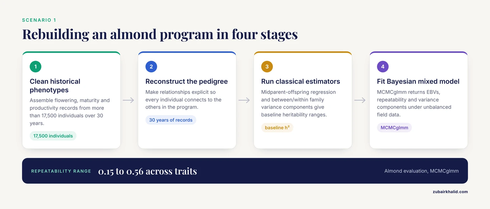
Four-stage flow for an almond program: clean historical phenotypes, rebuild the pedigree, run classical estimators, then fit a Bayesian mixed model.

Imagine inheriting an almond breeding program with decades of flowering, maturity, and productivity records but no unified pedigree. The realistic path runs through four stages. First, assemble and clean the historical phenotypes, which in the published case meant more than 17,500 individuals and over 30 years of records from a single breeding program [2]. Second, reconstruct the pedigree so relationships are explicit. Third, run classical estimators, midparent-offspring regression and between/within family variance components, to get baseline heritability ranges and a check on the data. Fourth, fit a Bayesian mixed model in MCMCglmm to obtain EBVs, repeatability, and variance components under the unbalanced structure that long-term field data always have [2]. The end product is a trait-specific ranking of every individual, including seedlings never phenotyped, refined by reliability, which lets the program discard weak material years before it would flower and fruit.

Scenario 2: Running a National Beef Evaluation

A national Nellore evaluation illustrates the industrial end of pedigree BLUP. The published workflow covered 954,216 animals with a pedigree of 1,348,164, and between roughly 227,000 and 532,000 records per trait across age at first calving, early pregnancy, scrotal circumference at 18 months, and total calvings at 53 months [5]. The decisive work happened before any model ran: defining contemporary groups, setting minimum group sizes, and choosing standard-deviation thresholds for removing phenotypic outliers, with alternative definitions compared by linear regression validation [5]. Continuous traits went through a linear animal model in the BLUPF90 family, while the binary pregnancy trait and the calving count went through a Bayesian threshold model in THRGIBBS1F90 [5]. The lesson scales down to any program size: editing decisions are not clerical, they change the EBVs.

Scenario 3: Adding Omics to Poultry Genomic Selection

A poultry breeding company weighing body-weight traits faces a cost question: is measuring gene expression worth it? The published evaluation used 350 Tiannong Partridge Chickens with whole-genome resequencing and pectoral muscle transcriptomes, then compared genomic-transcriptomic BLUP models under three data scenarios: transcriptomes in both reference and validation populations, in the reference only, or in neither, with the last case relying on a public reference panel to predict expression EBVs from SNPs [8]. Models incorporating predicted expression EBVs, whether from BLUP or elastic net prediction, competed against genomic-feature BLUP and standard genomic BLUP [8]. The practical takeaway is that predicted expression from reference panels offers a middle path, capturing some of the phenotype-proximity of transcriptomics without measuring transcriptomes on every bird [8].

Common Mistakes and Limitations

Reading an EBV as a promise. An EBV is an estimate with an error distribution, expressed relative to a defined base population. A sire with a top milk EBV can still produce daughters below the herd average if the estimate was imprecise or the environment differs.

Comparing numbers across evaluations or countries. Sire rankings on different national total merit indexes can diverge substantially, and countries update their genetic bases on different schedules, so index values are only comparable within one evaluation and one base [11].

Letting data editing happen by default. Contemporary group definitions, minimum group sizes, and outlier thresholds changed the results of a large-scale cattle evaluation [5]. Document every editing rule before the model runs.

Measuring traits inconsistently. Non-standard phenotyping quietly destroys comparability across years and sites. Published standardized protocols for core maize traits exist because consistent measurement is what allows phenotypic data to be integrated across experiments and programs [6].

Trusting pedigrees blindly. Genotypes expose pedigree errors through Mendelian inconsistency checks, and even the realized genomic relationships of full siblings deviate measurably from the pedigree expectation [7]. Verify parentage before the relationship matrix is built.

Discarding uncertainty. Selection on point-estimate EBVs gave up a measurable share of achievable genetic gain in simulation, while using the full posterior distribution preserved expected gain and protected the worst-case outcome [15]. If your calculator offers credible intervals, use them.

Expecting precision from low-heritability traits. When heritability is very low, as in some racing performance traits, even the best-supported model leaves wide uncertainty around each EBV [10]. Report reliability beside every published value.

Confusing repeatability with heritability. Repeatability measures consistency within individuals across repeated records and sets an upper bound on heritability, but the two answer different questions, and in long-term almond data they took distinctly different values across traits [2].

Overrunning a simple calculator's design limits. A midparent spreadsheet cannot handle unbalanced pedigrees, fixed effects, or genomic relationships, and forcing it to produces numbers that look precise and are not. Polyploid crops need adapted models as well, because inheritance patterns differ among tetraploid pummelo, mandarin, and the allotetraploid sour orange depending on their phylogenomic structure [16].

For the health or breeding status of an individual animal, involve a veterinarian or the evaluation center that runs the relevant program, because EBVs inform decisions, they do not replace them.

Choosing the Best Breeding Value Calculator for Your Data

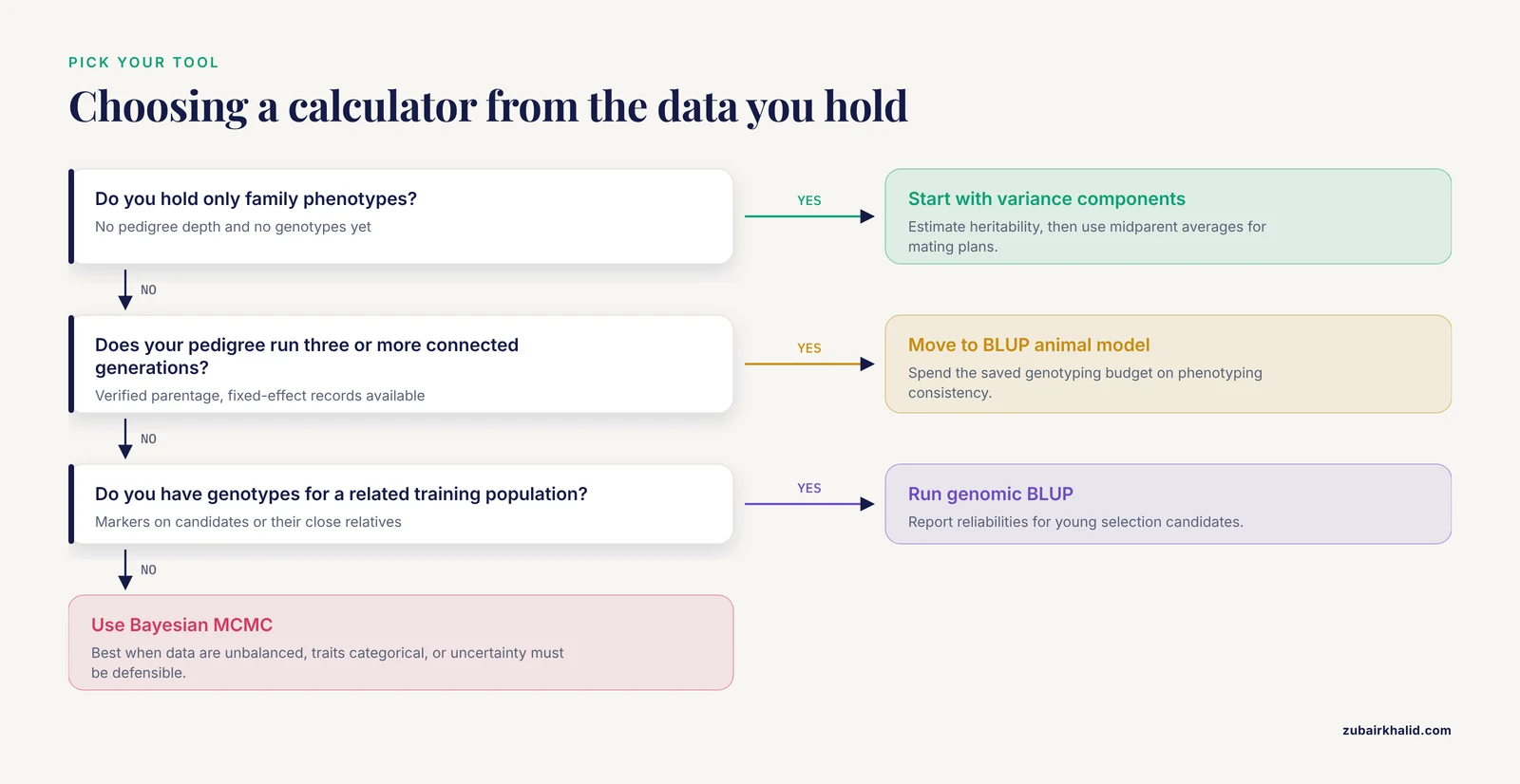
Decision path that starts from the records a breeder holds and ends at a recommended calculator family, from midparent regression to Bayesian MCMC.

Any genetic calculator for quantitative traits is only as good as its inputs, so treat the choice as a data audit before it is a software decision.

Inventory your records. Count phenotypes, verify pedigree depth, and check whether genotypes exist or could be budgeted.
If you hold only family phenotypes, start with a variance-component calculator to estimate heritability, then use midparent averages for planning matings.
If your pedigree runs three or more connected generations, move to a BLUP animal model and invest the saved genotyping budget in phenotyping consistency.
If genotypes exist for a training population related to your candidates, run genomic BLUP and report reliabilities for young selection candidates.
If your data are unbalanced, your traits are categorical, or you need defensible uncertainty, use a Bayesian MCMC model and carry the posterior into selection decisions.
Whatever the upstream calculator, finish with a selection index whose weights your breeding objective justifies, and re-estimate the weights when the objective changes.
Validate before you trust. Compare candidate models on prediction accuracy and bias, as the horse racing evaluation did across its alternative model structures [10], and re-validate when the population or the trait definition changes.

Frequently Asked Questions

What does a breeding value calculator do?

It estimates the breeding value, the additive genetic merit an individual is expected to pass to its offspring, for quantitative traits such as growth, yield, or flowering time. Inputs are phenotypes, pedigree, and sometimes genome-wide markers, and the output is an EBV with an accuracy or reliability attached.

Which is the best breeding value calculator for a small breeding program?

The best breeding value calculator is the one matched to the data you hold. With a few hundred family records, a spreadsheet-based midparent and variance-component calculator is appropriate and transparent. BLUP and genomic tools need pedigree depth or marker data before their extra complexity pays for itself.

Can a breeding value calculator work without genotyping?

Yes. Classical calculators need only family phenotypes, and pedigree-based BLUP runs on phenotypes plus a verified pedigree. Genotyping improves precision, especially for young animals with no records and for separating full siblings, but it is an upgrade, not a requirement.

How accurate are breeding value predictions?

Accuracy depends on trait heritability, the number of recorded relatives, and marker coverage, and every evaluation reports it alongside the EBV as accuracy or reliability. Low-heritability traits support much lower accuracy than high-heritability traits under the same data volume, so compare reliabilities before comparing animals.

What is the difference between an EBV and a phenotype?

A phenotype is what you measured on one individual in one environment. An EBV is the genetic merit estimated for that individual after adjusting for environmental effects and combining information from all recorded relatives.

What should I collect before running any genetic calculator for quantitative traits?

Collect consistently defined phenotypes, a verified pedigree or genotypes, records of management groups, seasons, and environments, and a written breeding objective with trait weights. Data quality at the input stage determines the ceiling on everything the calculator produces.