Pipette Calibration Uncertainty: How to Calculate
By Dr. Zubair Khalid, DVM, MS, PhD ·

By the end of this article you will be able to calibrate an air-displacement pipette gravimetrically, convert your weighings into delivered volumes, build a complete uncertainty budget, and report a final calibrated volume with an expanded uncertainty at roughly 95 percent confidence. You will also be able to judge whether the pipette still meets its manufacturer or ISO 8655 tolerance and decide whether it needs adjustment, repair, or retirement.
Here is what you need on hand before you start:
- An analytical balance readable to 0.1 mg (0.01 mg for pipettes below 100 µL), with a current calibration certificate
- A pipette, correctly sized tips, and a tip rack at room temperature
- Distilled or deionized water, degassed if it has been stored cold, held at 20 to 25 °C
- A thermometer readable to 0.5 °C, a barometer or local pressure record, and a hygrometer if available
- A weighing vessel (a small glass beaker or weighing boat with a lid to limit evaporation)
- A spreadsheet, or Python 3 with the standard library, for the arithmetic
Everything below follows the standard metrology framework described in the Guide to the Expression of Uncertainty in Measurement (the GUM), which underpins ISO 8655 piston-volume calibration practice. The general method is established textbook material. One published study, cited where its findings apply, shows exactly why this calculation matters in real quantitative assays.
Why Pipette Calibration Uncertainty Matters
A pipette that "dispenses 1000 µL" never dispenses exactly 1000 µL. It dispenses a volume that varies run to run and may sit slightly above or below the set value. Pipette calibration is the process of measuring the true delivered volume, and pipette calibration uncertainty is the quantified range around that measured value within which the true delivered volume probably lies.
This is not a paperwork exercise. In quantitative assays, the pipette is part of the measurement chain, and its uncertainty propagates into every downstream number. A study of ¹⁸F-FDG blood concentration measurement for dynamic PET analysis explicitly treated the precision of blood volume measured with a micropipette as a component of the overall measurement uncertainty, because errors in the sampled volume shift the estimated input function [1]. That same study compared three calibration strategies for the radiation detectors and found that a multiple-point calibration covering the full expected activity range gave the most accurate results, outperforming single-point calibration [1]. The same logic applies to pipettes. A pipette verified only at its nominal volume carries unquantified behavior at 10 percent and 50 percent of nominal, and a multi-point pipette calibration captures that behavior the way the multi-point detector calibration captured detector behavior [1].
When the pipette contributes an unknown amount of error, every concentration, every copy number, and every kinetic parameter calculated from your liquid handling inherits that unknown. When you quantify it, you can state your result as, for example, 1001.1 µL ± 0.4 µL, and defend it in an audit, a publication, or a method validation.
Vocabulary You Need Before Calculating
Each term below appears in the calculation itself, so define it once here.
Error is the difference between the measured value and the true value. If your 1000 µL setting actually delivers 1001.1 µL, the error is +1.1 µL. Error is a single number for a given pipette at a given setting.
Uncertainty is the range around a measured value that expresses the doubt about it. Unlike error, uncertainty cannot be corrected away. It describes the quality of your measurement of the error.
Accuracy describes closeness to the true value. Precision describes the spread of repeated results. A pipette can be precise (tight clustering) but inaccurate (clustered around 995 µL), and calibration corrects the accuracy problem while uncertainty describes how well you know the correction.
Standard uncertainty (u) expresses each uncertainty component as one standard deviation. It is the raw material of the calculation.
Type A evaluation derives a standard uncertainty from statistical analysis of repeated observations, typically the standard deviation of your replicate weighings divided by the square root of the number of weighings.
Type B evaluation derives a standard uncertainty from sources you cannot easily repeat, such as the balance calibration certificate, the balance readability, air buoyancy, and temperature. You evaluate these from certificates, specifications, and physical reasoning, usually assuming a rectangular (uniform) distribution where any value in an interval is equally likely.
Combined standard uncertainty (u_c) is the root sum of squares of all the standard uncertainty components, the standard GUM combination rule for independent inputs.
Expanded uncertainty (U) is u_c multiplied by a coverage factor. With k = 2, the interval covers approximately 95 percent of the distribution of possible values, and this is the conventional reporting choice.
Traceability means your balance calibration certificate traces through an unbroken chain of comparisons to a national standard, which is what makes your volume result defensible.
The Gravimetric Method for Pipette Calibration
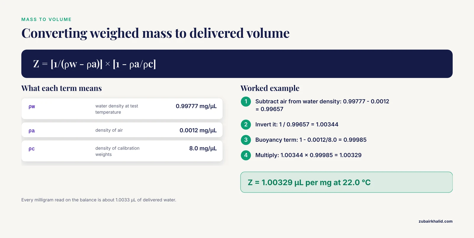
The gravimetric method is the standard approach in ISO 8655-6. You dispense water into a tared vessel on an analytical balance, record the mass, and convert mass to volume using the density of water at the test temperature, corrected for air buoyancy.
Why the buoyancy correction? The balance compares the weight of your water against the weight of calibration weights (typically stainless steel, density about 8.0 g/cm³). Both the water and the weights are buoyed by air (density about 0.0012 g/cm³ at sea level), but by different amounts because their densities differ. The raw mass reading is therefore slightly biased, and the correction factor Z accounts for it.
The conversion from mass to delivered volume is:
V = m × Z

where

Z = [1 / (ρw - ρa)] × [1 - ρa/ρc]

V  = delivered volume in µL
m  = apparent mass in mg (the balance reading)
ρw = density of water at the test temperature, in mg/µL
ρa = density of air, about 0.0012 mg/µL
ρc = density of the balance calibration weights, about 8.0 mg/µL
Because Z is dimensionless in effect (it converts mg to µL with the buoyancy factor folded in), the arithmetic is straightforward once you have the water density. Water density changes measurably with temperature, so you must use the value for your actual test temperature:
| Temperature (°C) | Density of water (g/mL) |
|---|---|
| 20.0 | 0.99820 |
| 21.0 | 0.99799 |
| 22.0 | 0.99777 |
| 23.0 | 0.99754 |
| 24.0 | 0.99730 |
| 25.0 | 0.99704 |
These are standard physical reference values. Interpolate between rows if your thermometer reads between listed temperatures. At 22.0 °C the Z factor works out to:
Z = [1 / (0.99777 - 0.0012)] × [1 - 0.0012/8.0]
  = [1 / 0.99657] × [1 - 0.00015]
  = 1.00344 × 0.99985
  = 1.00329 µL per mg
So every milligram the balance reads corresponds to about 1.0033 µL of delivered water, roughly a 0.33 percent correction that you cannot skip if you want an honest result.
The Pipette Calibration Uncertainty Calculation Formula
The full pipette calibration uncertainty calculation formula combines a Type A component with several Type B components. Written out:
u_c = sqrt( u_A² + u_balance² + u_read² + u_buoy² + u_temp² + u_evap² )

U = k × u_c          (k = 2 for approximately 95 % coverage)
Each component is evaluated as follows.
Type A, repeatability (u_A). Dispense n times (10 is the conventional minimum for a calibration point), calculate the standard deviation s of the converted volumes, and divide by √n:
u_A = (s / √n) × ZNote the √n. This gives the uncertainty of the mean, which is what a calibration reports. If you instead want the uncertainty of a single future dispensing by this pipette, use s × Z without dividing by √n, and say so explicitly in your documentation, because the two numbers differ by a factor of √10.
Balance calibration certificate (u_balance). Take the expanded uncertainty stated on the certificate at the relevant load, divide by its stated coverage factor (usually 2). If the certificate states U = 0.10 mg at k = 2, then u_balance = 0.05 mg, converted to µL with Z.
Balance readability (u_read). A digital balance of resolution d has a rounding uncertainty treated as rectangular: u = (d/2)/√3 = d/(2√3). For d = 0.01 mg, u_read ≈ 0.0029 mg.
Air buoyancy (u_buoy). Air density varies with pressure, temperature, and humidity. In an air-conditioned laboratory, assume the actual air density may differ from the assumed 0.0012 mg/µL by roughly 10 percent. The sensitivity of volume to air density is approximately ΔV ≈ m × Δρa/(ρw - ρa). Divide the resulting worst-case shift by √3 for the rectangular distribution.
Water temperature (u_temp). If your thermometer reads to ±0.5 °C, the water density uncertainty is about 0.00025 mg/µL per °C × 0.5 °C = 0.000125 mg/µL. The relative volume effect is Δρw/(ρw - ρa), applied to the measured volume, divided by √3.
Evaporation and drift (u_evap). Water evaporates from the weighing vessel between dispensings, which biases masses downward and adds scatter. With a covered vessel and minimal exposure, a conservative estimate for a 1 mL dispense is on the order of 0.1 µL worst case, treated as rectangular (divide by √3). This is a laboratory-specific estimate, and you should scale it to your own vessel geometry and exposure time.
The table below summarizes the components, their evaluation method, and the example values used in the worked example for a 1000 µL nominal setting.
| Component | Type | Distribution | How to evaluate | Example value (1 mL) |
|---|---|---|---|---|
| Repeatability of dispensing and weighing | A | Normal | (s/√n) × Z from 10 weighings | 0.153 µL |
| Balance calibration certificate | B | Normal (k = 2) | certificate U ÷ 2 | 0.050 µL |
| Balance readability | B | Rectangular | d ÷ (2√3) | 0.003 µL |
| Air buoyancy | B | Rectangular | sensitivity × Δρa ÷ √3 | 0.069 µL |
| Water temperature and density | B | Rectangular | (dρ/dT × ΔT) ÷ (ρw - ρa) × V ÷ √3 | 0.072 µL |
| Evaporation and drift | B | Rectangular | lab-specific worst case ÷ √3 | 0.058 µL |
How to Calculate Pipette Calibration Uncertainty, Step by Step
Follow these ten steps in order. Steps 1 through 4 are bench work, steps 5 through 10 are arithmetic you can automate.
Step 1. Prepare the environment
Place the balance on a stable, vibration-free surface, level it, and let it warm up per the manufacturer's instructions. Record room temperature, and let the water, pipette, and tips equilibrate to room temperature for at least an hour. Temperature mismatch between the pipette, the tip, and the liquid is one of the largest avoidable error sources in gravimetric work. Record the barometric pressure if you want to refine the air density term. Drafts, direct sunlight, and hand heat on the weighing vessel all bias small mass readings, so work calmly with the balance draft shield closed between additions.
Step 2. Choose the test volumes
Calibrate at a minimum of three settings across the pipette range, conventionally 10 percent, 50 percent, and 100 percent of nominal volume. A single nominal-volume check hides the fact that most air-displacement pipettes perform worst at the bottom of their range. The multi-point logic mirrors the finding in the ¹⁸F measurement study that calibrating across the full working range produced more accurate results than a single calibration point [1].
Step 3. Perform the replicate weighings
For each test volume: place the weighing vessel on the balance, tare, pre-rinse the tip by aspirating and dispensing the test liquid three times, then dispense ten replicate volumes into the vessel, recording the mass after each. Keep the pipette vertical, immerse the tip 2 to 3 mm into the liquid during aspiration, and deliver against the vessel wall with a smooth press to the first stop followed by full blow-out. Tare between replicates or track cumulative mass, whichever your balance software supports. Ten replicates per point is the standard minimum because it stabilizes the standard deviation estimate.
Step 4. Record conditions
Write down the test temperature, the balance ID and certificate number, the pipette serial number, the tip lot, and the operator. An uncertainty calculation without these identifiers cannot be traced or reproduced.
Step 5. Compute the mean mass and standard deviation
For each test volume, calculate the mean and sample standard deviation of the ten mass readings. In Excel, with masses in cells B2 through B11:
=AVERAGE(B2:B11)
=STDEV.S(B2:B11)
In Python:
import statistics

masses_mg = [997.5, 998.2, 997.1, 998.6, 997.9,
             997.3, 998.4, 997.7, 998.0, 997.6]

mean_mg = statistics.mean(masses_mg)
s_mg = statistics.stdev(masses_mg)
Step 6. Convert mass to volume
Multiply the mean mass by the Z factor for your test temperature. Using 22.0 °C, Z = 1.00329 µL/mg.
Step 7. Calculate the Type A standard uncertainty
Divide the standard deviation of the masses by √n, then multiply by Z. This is the uncertainty of your calibrated mean volume.
Step 8. Assemble the Type B components
Pull the balance certificate value, the balance resolution, your air density allowance, your thermometer tolerance, and your evaporation estimate, convert each to a standard uncertainty as described in the formula section, and express everything in µL at the same test volume.
Step 9. Combine and expand
Square each component, sum, take the square root to get u_c, and multiply by 2 for the expanded uncertainty U.
Step 10. Report
Report the result as: calibrated volume = mean ± U (k = 2), plus the test conditions. For example, 1001.1 µL ± 0.4 µL (k = 2), which reads as the delivered volume lies between 1000.7 and 1001.5 µL with approximately 95 percent confidence.
A Worked Example with Real Numbers
Here is a complete pipette calibration uncertainty calculation worked example for a single-channel pipette set to 1000 µL, tested with ten gravimetric replicates at 22.0 °C on a 0.1 mg balance with 0.01 mg readability and a certificate stating U = 0.10 mg at k = 2.
The ten apparent masses, in mg, were 997.5, 998.2, 997.1, 998.6, 997.9, 997.3, 998.4, 997.7, 998.0, and 997.6.
import statistics

# Step 5: descriptive statistics of the ten weighings
masses_mg = [997.5, 998.2, 997.1, 998.6, 997.9,
             997.3, 998.4, 997.7, 998.0, 997.6]

n = len(masses_mg)
mean_mg = statistics.mean(masses_mg)
s_mg = statistics.stdev(masses_mg)

# Step 6: conversion factor at 22.0 C
rho_w = 0.99777      # water density, mg per uL
rho_air = 0.0012     # air density, mg per uL
rho_weights = 8.0    # calibration weight density, mg per uL

Z = (1 / (rho_w - rho_air)) * (1 - rho_air / rho_weights)

mean_uL = mean_mg * Z
u_A = (s_mg / (n ** 0.5)) * Z

# Step 8: Type B components, all converted to uL
u_balance = 0.10 / 2          # certificate U = 0.10 mg at k = 2
u_read = 0.01 / (2 * 3 ** 0.5)  # resolution 0.01 mg, rectangular
u_buoy = 0.12 / 3 ** 0.5      # air density allowance, rectangular
u_temp = 0.126 / 3 ** 0.5     # thermometer tolerance effect, rectangular
u_evap = 0.10 / 3 ** 0.5      # evaporation estimate, rectangular

# Step 9: combination and expansion
u_c = (u_A**2 + u_balance**2 + u_read**2 +
       u_buoy**2 + u_temp**2 + u_evap**2) ** 0.5
U = 2 * u_c

print(f"mean volume = {mean_uL:.2f} uL")
print(f"s (mass)    = {s_mg:.3f} mg")
print(f"Z           = {Z:.5f}")
print(f"u_A         = {u_A:.3f} uL")
print(f"u_c         = {u_c:.3f} uL")
print(f"U (k = 2)   = {U:.2f} uL")
print(f"relative U  = {100 * U / mean_uL:.3f} %")
Run the script and you get the expected output:
mean volume = 1001.12 uL
s (mass)    = 0.481 mg
Z           = 1.00329
u_A         = 0.153 uL
u_c         = 0.199 uL
U (k = 2)   = 0.40 uL
relative U  = 0.040 %
Interpretation. The pipette delivers a mean of 1001.1 µL at the 1000 µL setting, a systematic error of +1.1 µL or +0.11 percent. You know this value to within ±0.4 µL at approximately 95 percent confidence. If you prefer the same budget expressed for a single future dispensing rather than the calibrated mean, drop the √n in u_A, which raises u_A to 0.483 µL and U to roughly 1.0 µL. Both numbers are correct. They answer different questions, and your report must say which one you are quoting.
The same calculation in Excel, with the ten masses in B2:B11 and the constants in named cells, looks like this:
B13: mean mass (mg)        =AVERAGE(B2:B11)
B14: SD of mass (mg)       =STDEV.S(B2:B11)
B15: Z factor              =(1/(0.99777-0.0012))*(1-0.0012/8)
B16: mean volume (uL)      =B13*B15
B17: u_A (uL)              =B14/SQRT(10)*B15
B18: u_balance (uL)        =0.10/2*B15
B19: u_read (uL)           =0.01/(2*SQRT(3))*B15
B20: u_buoy (uL)           =0.12/SQRT(3)
B21: u_temp (uL)           =0.126/SQRT(3)
B22: u_evap (uL)           =0.10/SQRT(3)
B23: u_c (uL)              =SQRT(B17^2+SUMPRODUCT(B18:B22,B18:B22))
B24: U, k = 2 (uL)         =2*B23
For a smaller pipette, say 100 µL or 10 µL, the same structure applies but the balance becomes the limiting factor. A 0.1 mg balance cannot resolve a 10 µL dispense with meaningful relative uncertainty, which is why ISO 8655 practice calls for a 0.001 mg (1 µg) readability balance for low-volume piston-operated apparatus. Check that your balance certificate uncertainty is small relative to your Type A component. If it is not, no amount of extra replicates will rescue the budget, because the Type B floor dominates.
Judging the Result Against Tolerances
Calibration and uncertainty answer two different questions, and confusing them is the most common analytical mistake. The calibrated mean volume (1001.1 µL) and its expanded uncertainty (±0.4 µL) describe what you measured. The tolerance describes what the pipette is allowed to do.
ISO 8655-2 sets limits for air-displacement pipettes. At the 1000 µL nominal setting, the maximum permissible systematic error is about ±8 µL and the maximum permissible repeatability limit is about ±3 µL for the standard accuracy class. Your worked example sits at +1.1 µL systematic with a repeatability standard deviation of 0.48 µL, comfortably inside both limits. The pass criterion in routine calibration is that the systematic error falls within the tolerance and the repeatability falls within its limit, evaluated with the uncertainty in mind. If your measured error is smaller than your expanded uncertainty, you cannot honestly claim the pipette is out of tolerance even if the mean sits slightly off nominal, because the measurement itself cannot distinguish the error from zero with the confidence you claim. This judgment call, error versus uncertainty, is the heart of a defensible go/no-go decision.
Common Mistakes and Limitations
- Reporting the standard deviation as the uncertainty. The standard deviation of your ten weighings (0.48 µL in the example) is a repeatability figure, not the expanded uncertainty of the calibration. Conflate them and your reported uncertainty is wrong by roughly a factor of five in the example, after ignoring the Type B terms.
- Forgetting the √n, or applying it twice. The Type A uncertainty of the mean includes √n. If you also average several calibration sessions and then divide again, you have double-counted averaging. Decide what quantity the calibration represents (the mean delivered volume today) and apply the statistics once.
- Double counting the balance. Balance repeatability shows up inside your Type A component, because every weighing includes it. Adding a separate balance repeatability Type B term inflates the budget. Only add a Type B balance term if your Type A came from dispensing replicates weighed on a different instrument or from historical data.
- Using water density tables for other liquids. The Z factor above is valid for water. Ethanol, buffer, and solvent calibrations need different densities and often a different evaporation model. Using the water table for 70 percent ethanol understates the delivered volume by close to its density difference, over 10 percent.
- Calibrating only at nominal volume. Bottom-of-range performance is where air-displacement pipettes degrade first. A single-point check misses this, which is the same lesson the multi-point versus single-point calibration comparison in the ¹⁸F study teaches [1].
- Static and drafts on plastic vessels. Plastic weighing boats carry static charge and drift the balance. Glass vessels, an antistatic ionizer, and a closed draft shield fix most mystery drift.
- Ignoring evaporation with small volumes. At 10 µL per dispense, evaporation during a ten-replicate series is a significant fraction of the volume. Work quickly, use a covered vessel, and increase the evaporation term honestly.
- Rounding too early or too much. Carry full precision through the calculation and round only the final U, conventionally to two significant figures, then round the mean to match the last digit of U.
- Treating a calibration certificate uncertainty as zero. Even a recently calibrated balance carries a stated uncertainty. Omitting it flatters your result and is the first thing an assessor checks.
One limitation to state plainly. The numerical component values in the worked example reflect one plausible laboratory setup. Your balance certificate, your thermometer tolerance, and your evaporation conditions differ, so you must substitute your own Type B values. The formula structure does not change.
How Pipetting Technique Affects the Uncertainty Budget
Your pipetting technique feeds directly into the Type A component, because every source of run-to-run variation, whether it comes from the pipette, the tip, the liquid, or your hands, lands in the same standard deviation. The published ¹⁸F work made this concrete by evaluating micropipette volume precision through repeated blood sampling rather than through the pipette specification sheet alone, treating the operator and the workflow as part of the measurement system [1].
Technique factors worth controlling:
- Pre-rinsing the tip. For aqueous solutions, one to three pre-rinses condition the tip surface and improve consistency, particularly below 100 µL.
- Immersion depth. Aspirate with the tip 2 to 3 mm below the liquid surface. Too deep and liquid coats the outside, too shallow and you risk aspirating air.
- Vertical holding. Hold the pipette within about 20 degrees of vertical during aspiration. Pocket-carrying a pipette at an angle shifts the hydrostatic head and biases the aspirated volume.
- Smooth plunger speed. Aspirate slowly and consistently. Fast aspiration creates aerosols and splashing inside the tip, and slow inconsistent release leaves variable residual volumes.
- Forward versus reverse pipetting. Forward pipetting (to the first stop for aspiration, full blow-out for delivery) suits aqueous solutions. Reverse pipetting (aspirate to the second stop, dispense to the first stop, leave the excess in the tip) suits viscous or foaming liquids. Switching modes mid-series without noting it will appear in your standard deviation.
- Consistent operator. If multiple operators perform the calibration, expect the Type A component to reflect operator-to-operator variation. That is legitimate, but record it, and do not mix a trained operator's ten replicates with a new operator's ten without noting the design.
If your Type A component comes out far larger than the manufacturer's repeatability specification for the pipette, the pipette is usually not the problem. Your technique, your tips, or your environment is.
Frequently Asked Questions
What is pipette calibration uncertainty?
Pipette calibration uncertainty is the quantified range around a pipette's calibrated delivered volume that expresses how well you know that volume. It combines the statistical spread of your replicate weighings (Type A) with non-statistical contributions from the balance, buoyancy, temperature, and evaporation (Type B), and is reported as an expanded uncertainty U = k × u_c, conventionally with k = 2.
What is the pipette calibration uncertainty calculation formula?
The core formula is u_c = √(u_A² + u_balance² + u_read² + u_buoy² + u_temp² + u_evap²), and U = k × u_c with k = 2. The volume itself comes from V = m × Z, where Z = [1/(ρw - ρa)] × [1 - ρa/ρc]. Each component is converted to a standard uncertainty in µL before combination.
How many weighings do I need for a valid uncertainty calculation?
Ten replicate weighings per test volume is the conventional minimum, because it gives a reasonably stable standard deviation estimate for the Type A component. Fewer than five makes the standard deviation itself unreliable, and more than ten gives diminishing returns unless you are chasing an instability you suspect is real.
What kind of balance do I need to calibrate a pipette?
You need an analytical balance with readability of at least 0.1 mg for pipettes of 100 µL and above, and 0.001 mg or better for pipettes below 100 µL, with a current traceable calibration certificate. The certificate's stated uncertainty must be small relative to the volume you are measuring, or it will dominate your Type B budget.
What is the difference between error and uncertainty?
Error is the signed difference between the measured delivered volume and the nominal setting, and it can be corrected. Uncertainty is the range of doubt around your measured value, and it cannot be corrected away. In the worked example, the error is +1.1 µL and the expanded uncertainty is ±0.4 µL at k = 2.
How often should a pipette be calibrated?
Most laboratories recalibrate pipettes on a 6 to 12 month cycle, with intermediate checks between full calibrations. The appropriate interval depends on usage frequency, the liquids handled, the criticality of the assays, and the pipette's drift history, so shorten the interval for heavily used or corrosive-service pipettes and lengthen it for lightly used ones with a stable record.
Does pipetting technique really change the calculated uncertainty?
Yes. Every source of run-to-run variation, including inconsistent plunger speed, variable immersion depth, angled holding, and skipped pre-rinsing, appears in your replicate standard deviation and therefore inflates the Type A component. A Type A result far worse than the manufacturer's repeatability specification usually points to technique or tips rather than the pipette mechanism.
What is a coverage factor and why is k = 2?
A coverage factor multiplies the combined standard uncertainty to widen the interval to a stated confidence level. k = 2 gives approximately 95 percent coverage under the near-normal conditions of a calibration budget, so reporting 1001.1 µL ± 0.4 µL (k = 2) means the true delivered volume lies within 1000.7 to 1001.5 µL with about 95 percent confidence. Use k = 1 only when you explicitly want to report a standard uncertainty, and say so.