Chargaff's Rule: Base Pairing Explained with Examples
By Dr. Zubair Khalid, DVM, MS, PhD ·
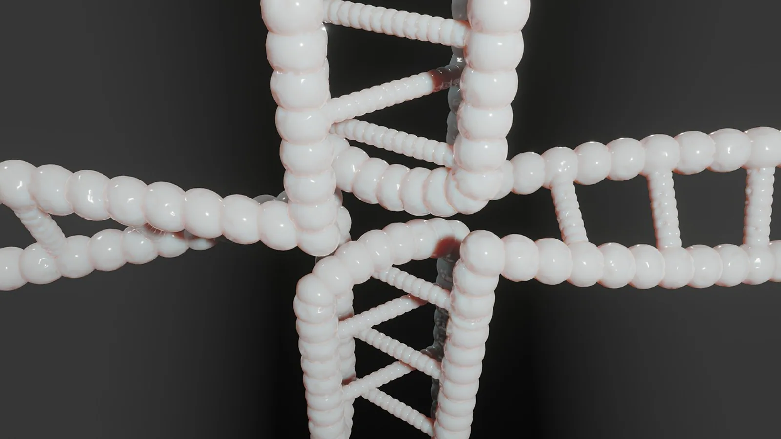
Chargaff's rule states that in double-stranded DNA the amount of adenine equals the amount of thymine (%A = %T) and the amount of guanine equals the amount of cytosine (%G = %C), so the total purines equal the total pyrimidines. A second, related rule states that these equalities also hold approximately within a single strand of most genomes, even though a single strand has no physical partner to pair with.
Those two facts connect the chemistry of the double helix to the arithmetic of a sequencing report. If a lab tells you a DNA sample is 30% adenine, you can immediately pencil in 30% thymine, subtract 60 from 100, and split the remaining 40% evenly between guanine and cytosine. No gel, no sequencer, no alignment. The rule also explains why the Watson-Crick model fit the data so well: antiparallel strands with A paired to T and G paired to C automatically produce the equalities Erwin Chargaff measured, and the model would have been wrong if those equalities did not appear.
The Two Chargaff Rules
Most textbooks compress Chargaff's finding into one sentence, but there are genuinely two rules, and they are not the same statement.
The first parity rule
The first parity rule applies to the duplex as a whole. Count every adenine in both strands and every thymine in both strands, and the two numbers match. The same holds for guanine and cytosine. This is exact within the limits of measurement, because every A on one strand sits across from a T on the other, and every G sits across from a C.
This rule is a direct consequence of Watson-Crick geometry, not an independent law of nature. If you built a duplex that paired A with C and G with T, you would get different equalities.
The second parity rule
The second parity rule states something stranger. Take a single strand, ignore its partner, and count bases along that strand alone. In most genomes, %A still approximately equals %T and %G still approximately equals %C within that one strand [1]. The same near-equality extends beyond single bases to short oligonucleotides, so the frequency of a k-mer roughly matches the frequency of its reverse complement on the same strand [2]. This version is often called intra-strand parity or strand symmetry.
The second rule is not forced by base pairing. A single strand is free to contain any sequence, so the near-equality must come from how genomes evolve, mutate, and rearrange rather than from hydrogen bonding. Several explanations have been proposed: mutation-rate interrelations that push complementary substitutions toward balance [3], recombination-driven strand exchange including inversions and inverted transpositions [2], and structural pressures that favor the potential for both strands to extrude stem-loop structures [4]. A maximum-entropy argument holds that some of the symmetry emerges from the physical constraints of the duplex itself rather than from selection [5]. These explanations are not mutually exclusive.
A summary of the two rules
| Feature | First parity rule | Second parity rule |
|---|---|---|
| What is compared | A vs T, G vs C across both strands of a duplex | A vs T, G vs C within a single strand |
| Accuracy | Exact within measurement error | Approximate, improves with segment length |
| Physical basis | Watson-Crick base pairing | Evolutionary, mutational, and structural processes |
| Applies to single-stranded genomes | Not applicable | Usually fails |
| Applies to mitochondrial DNA | Yes | Often fails |
Base Pairing: The Chemistry Behind the Arithmetic
A DNA base pair is a hydrogen-bonded partnership between a purine and a pyrimidine. Purines are the two-ring bases, adenine (A) and guanine (G). Pyrimidines are the single-ring bases, thymine (T) and cytosine (C). Pairing a big base with a small base keeps the width of the helix constant, which is why the sugar-phosphate backbones run parallel at a fixed distance.
Adenine pairs with thymine
Adenine and thymine form two hydrogen bonds. Adenine presents an amino group and a ring nitrogen, thymine presents a carbonyl oxygen and a ring NH, and the geometry lines up so that two hydrogen bonds form. The A-T pair is sometimes written as A=T in shorthand, with the equals sign standing for the two bonds.
Guanine pairs with cytosine
Guanine and cytosine form three hydrogen bonds. The extra bond comes from the pattern of donors and acceptors on the Watson-Crick faces of the two bases. G-C pairs are therefore more stable than A-T pairs, which is why a DNA molecule with high GC content requires more energy to melt apart. This is standard duplex thermodynamics and underlies the melting-temperature calculations used in every PCR lab.
The pairing table
| Base pair | Base types | Hydrogen bonds | Shorthand | Relative duplex stability |
|---|---|---|---|---|
| A-T | Purine + pyrimidine | 2 | A=T | Lower |
| T-A | Pyrimidine + purine | 2 | T=A | Lower (same pair, flipped) |
| G-C | Purine + pyrimidine | 3 | G≡C | Higher |
| C-G | Pyrimidine + purine | 3 | C≡G | Higher (same pair, flipped) |
Why the pairing produces Chargaff's equalities
Every A on the top strand is bonded to a T on the bottom strand. Every G on the top strand is bonded to a C on the bottom strand. Now count: the total number of A residues in the duplex equals the number of A residues on the top strand plus the number on the bottom strand. The number of A on the top strand equals the number of T on the bottom strand, because each one is paired. The number of A on the bottom strand equals the number of T on the top strand. Add the two equations and the total A equals the total T. The same argument gives G = C. Nothing else is needed.
Worked Calculations with Percentages
These calculations show up constantly in exams and in real lab work, so it is worth doing several by hand.
Example 1: Given %A, find everything else
Suppose a double-stranded DNA sample is 30% adenine by base count.
Step 1. Apply the first parity rule to thymine. %T = %A = 30%.
Step 2. Add the A-T contribution. 30% + 30% = 60% of all bases are A or T.
Step 3. The remaining bases must be G and C. 100% - 60% = 40%.
Step 4. Apply the first parity rule to G and C, which must be equal. %G = %C = 40% ÷ 2 = 20%.
The full composition is A = 30%, T = 30%, G = 20%, C = 20%.
Example 2: Given %G, work backward
Suppose a sample is 22% guanine.
Step 1. %C = %G = 22%.
Step 2. G + C = 44%.
Step 3. A + T = 100% - 44% = 56%.
Step 4. %A = %T = 56% ÷ 2 = 28%.
Composition: A = 28%, T = 28%, G = 22%, C = 22%.
Example 3: Given %A + %T combined
Suppose a sample has 70% of its bases as A or T.
Step 1. %A = %T = 70% ÷ 2 = 35%.
Step 2. G + C = 30%.
Step 3. %G = %C = 15%.
Example 4: A purine and pyrimidine cross-check
Suppose a sample is 27% A and 27% G. Because %T = %A = 27% and %C = %G = 27%, the four bases each contribute 27%, which sums to 108%, an impossible result. The data must be wrong. Total purines (A + G) would be 54%, and total pyrimidines (T + C) would be 54%, which is consistent with the purine-pyrimidine parity but not with a full composition. This kind of arithmetic check is a standard way to catch a bad spectrophotometric reading or a mislabeled dataset.
Example 5: The GC content shortcut
GC content is defined as %G + %C, which is also 2 × %G. If a duplex is 30% A, then GC content = 40%. If a duplex is 28% A, GC content = 44%. Because %A = %T, you can always write GC content as 100% - 2(%A). For a 30% A sample this gives 100% - 60% = 40%, matching Example 1.
Example 6: Mole fraction versus percent
If a duplex contains 3,000 adenine residues, it contains 3,000 thymine residues. If the molecule is 10,000 base pairs long, it has 20,000 bases total. Then %A = 3,000 ÷ 20,000 = 15%, and the same arithmetic applies as before. Always check whether "amount" refers to a count, a mole fraction, or a percentage, because mixing units is the most common source of errors.
Example Organisms: Base Composition Table
The numbers below illustrate the range of base compositions seen across double-stranded genomes. Values are rounded and are meant as teaching examples of the sort of composition that a sequencing or chemical analysis produces, not as primary measurements from a specific citation. Use them to practice the calculations above.
| Example | %A | %T | %G | %C | GC content | Notes |
|---|---|---|---|---|---|---|
| Generic human genomic DNA | 29.5 | 29.5 | 20.5 | 20.5 | 41 | Typical mammalian GC level |
| GC-rich bacterial genome | 20.0 | 20.0 | 30.0 | 30.0 | 60 | Common in some soil bacteria |
| AT-rich bacterial genome | 30.0 | 30.0 | 20.0 | 20.0 | 40 | AT-rich genomes tend to be smaller |
| Thermophile-like composition | 15.0 | 15.0 | 35.0 | 35.0 | 70 | High GC correlates with thermal stability |
| Hypothetical duplex with 30% A | 30.0 | 30.0 | 20.0 | 20.0 | 40 | Worked example from the text |
Two patterns are worth memorizing. First, in every row %A = %T and %G = %C. Second, as GC content rises, A and T fall together, not separately.
Why GC content varies by organism
Base composition is a species-specific property that reflects genome-wide evolutionary pressure rather than a single environmental variable [6]. Thermophile base compositions were once taken as evidence for a neutral explanation of Chargaff's second rule, but GC content plays roles in both maintaining species integrity and generating variation during speciation, so it cannot be a simple thermometer reading [6]. In plants, ecological nitrogen limitation has been linked to base composition as well, with transcribed regions showing the strongest deviations from intra-strand parity [7]. Genome length and GC content show a complex relationship rather than a simple linear one [8].
Testing Chargaff's Rule in Practice
You do not need a sequencer to observe Chargaff's rule. Several classical and modern methods report base composition directly.
Chemical and spectroscopic methods
Early work by Chargaff relied on paper chromatography and ultraviolet spectrophotometry to separate and quantify the bases. UV absorbance at 260 nm is still used today to estimate total nucleic acid concentration, and the ratio of absorbance at 260 nm to 280 nm gives a purity check. These methods measure total bases, not sequence, so they are a natural fit for testing the first parity rule.
Sequencing-based composition analysis
Modern genome assembly pipelines count every base and report composition as standard output. You can compute %A = %T and %G = %C directly from any assembled double-stranded genome. The same calculation for the second parity rule requires you to split the assembly into its two strands, which many tools will do automatically. Standard file formats such as FASTA and GenBank store the sequence of one strand only, so strand-specific analysis requires either the reverse complement or tools that handle both orientations.
Melting curve analysis
Because G-C pairs have three hydrogen bonds and A-T pairs have two, melting temperature tracks GC content. If two DNA samples have identical GC content, their melting behavior should be similar under the same salt and buffer conditions. This gives an experimental cross-check on the composition inferred from the first parity rule.
K-mer and oligonucleotide analysis
At a finer level, you can count each trinucleotide and compare it with its reverse complement on the same strand. Genomes across a wide range of species, from bacteria to humans, comply closely with the triplet version of the second rule, with mitochondria as a notable exception class [2]. Trinucleotide quadruplet analysis has been used to show mirror symmetries across chromosomes of organisms from Escherichia coli to humans [9]. Software tools for k-mer counting and sequence-symmetry analysis are readily available, and any student can run them on a downloaded genome.
Chargaff's Data and the Watson-Crick Model
Erwin Chargaff's base composition measurements came before the double helix was solved, and they provided one of the key constraints that any correct model had to satisfy. Watson and Crick's model, once built, produced the equalities naturally: pair a purine with a pyrimidine, make A pair only with T and G pair only with C, and the totals come out even. If the data had shown %A not equal to %T, the model would have been dead on arrival.
The historical sequence matters for another reason. Chargaff's data supported the model but did not, on its own, determine the structure. The equalities are compatible with several possible hydrogen-bonding schemes. What made the Watson-Crick model correct was the combination of the equalities, the X-ray fiber diffraction pattern, and the geometry of the bases. This is why citing the rule as if it discovered base pairing is a mistake.
Comparative and Functional Relevance
Base composition is not just bookkeeping. It has direct consequences for several molecular and clinical contexts.
PCR primer design
The GC content of a primer determines its melting temperature and its tendency to form secondary structures. A primer with 60% GC will have a higher melting temperature than one with 40% GC, all else equal, because of the extra hydrogen bond in each G-C pair. The first parity rule tells you that raising GC content necessarily lowers AT content, so you cannot independently tune AT stability without affecting GC stability.
Genome stability and thermal adaptation
GC-rich genomes tend to be more thermally stable, which is why high-GC compositions show up in thermophiles and in organisms that live in high-temperature environments. This is a correlation, not a universal law, and exceptions exist.
Recombination and genome evolution
The second parity rule has been tied to meiotic recombination and the potential for single strands to extrude into stem-loop structures. Deviations from the rule appear near microsatellites and telomeres, where base order asymmetry is greatest [10]. Deviations also correlate with transcription direction in E. coli, Saccharomyces cerevisiae, and vaccinia virus, with the mRNA-synonymous strand showing characteristic base enrichment patterns [11]. Coding regions in humans violate the second parity rule in ways consistent with the existence of both purine-pyrimidine symmetry and sequence-specific constraints [12]. Nitrogen limitation in plants has been linked to the composition of transcribed regions as well [7].
Gene expression and codon usage
The second parity rule has been proposed as a factor underlying additive genetic interactions in quantitative traits, with implications for how polygenic selection operates [13]. Genomes that comply strictly with the second rule tend to show compositional equilibrium, while genomes that deviate, such as certain mitochondrial and viral genomes, have distinct evolutionary dynamics.
Common Mistakes and Limitations
Mistake 1: Thinking Chargaff's rule predicts sequence order
The rule tells you the proportions of bases, not their order. A 30% A duplex can have adenines spaced evenly, clustered in runs, or arranged in any pattern, and the composition is unchanged. Sequence is a separate question, and the second parity rule extends the composition symmetry to short words but never to full sequence identity.
Mistake 2: Thinking the two rules apply everywhere
The first parity rule holds for any double-stranded DNA that obeys Watson-Crick pairing. The second parity rule holds approximately in most nuclear genomes and fails or weakens in several important cases, including single-stranded viral genomes, certain mitochondria, and coding regions under strong directional selection [12][2].
Mistake 3: Assuming %A = %T implies %G = %C in any single strand
In a single strand, the two equalities can drift independently. A strand may be near parity for A and T but strongly biased for G and C, or vice versa.
Mistake 4: Confusing base composition with GC content
GC content is a useful summary, but it hides AT composition. Two genomes with identical GC content can have very different purine-pyrimidine balances, and the second parity rule is about the individual base equalities, not the summary figure.
Mistake 5: Ignoring single-stranded viral genomes
Single-stranded DNA viruses, such as those in the parvovirus family, carry one strand through much of their life cycle. The first parity rule is not meaningful for the packaged genome because there is no complementary strand present, and the second parity rule frequently fails because there is no duplex to average out strand bias. RNA viruses have uracil in place of thymine and are outside the classical formulation entirely.
Mistake 6: Forgetting that intra-strand parity improves with length
Short segments can deviate substantially from the second rule. The parity relationship stabilizes as segment length grows, because the sequence segments with opposite-sign biases are intermingled and average out [1]. Because of this, a short contig may look like an exception even though the full chromosome complies.
Mistake 7: Treating the second rule as fully solved
The mechanism behind the second parity rule remains actively debated, and no single explanation has displaced the others [4][14]. Students should know the phenomenon and the leading explanations, not just the statement.
Limitations and individual cases
Genomes and samples vary. If you are interpreting a specific sequencing dataset or a clinical assay result, the general rules in this article provide a framework, but the details of your sample, your organism, and your quality metrics matter. For veterinary or clinical interpretation of a particular animal or patient, a qualified professional should be involved.
Quick Review
- First parity rule: %A = %T and %G = %C in double-stranded DNA, accounting for both strands.
- Second parity rule: %A ≈ %T and %G ≈ %C within a single strand in most genomes, with exceptions.
- A pairs with T using two hydrogen bonds. G pairs with C using three hydrogen bonds.
- Given %A = 30, then %T = 30, G + C = 40, so %G = %C = 20.
- GC content = 100% - 2(%A) for a duplex that obeys the first rule.
- The rule fixes proportions, not sequence order.
- The second parity rule weakens in single-stranded viral genomes, some mitochondria, and coding regions under strong selection.
Frequently Asked Questions
What is Chargaff's rule in simple terms?
In double-stranded DNA, the percentage of adenine equals the percentage of thymine and the percentage of guanine equals the percentage of cytosine. This happens because A always pairs with T and G always pairs with C.
What is the difference between the first and second parity rules?
The first parity rule applies to the whole duplex and is exact. The second parity rule applies within a single strand and is approximate in most genomes, with clear exceptions.
How do you calculate %G and %C if %A is 30?
If %A = 30, then %T = 30, so A + T = 60. The remaining 40% is split evenly, giving %G = 20 and %C = 20.
How many hydrogen bonds form in each DNA base pair?
A-T pairs form two hydrogen bonds and G-C pairs form three. The extra bond makes G-C pairs more stable and raises the melting temperature of GC-rich DNA.
Does Chargaff's rule apply to single-stranded DNA and RNA?
The first parity rule does not apply to single-stranded genomes because there is no complementary strand to pair with. RNA uses uracil in place of thymine and is outside the classical formulation.
Does Chargaff's rule tell you the order of bases?
No. The rule constrains base proportions only. Sequence order is determined by the genome itself and cannot be recovered from composition alone.
Related Articles
- Purine Always Pairs with Pyrimidine: Base Pairing Rules
- RNA Base Pairs: A-U and G-C Pairing Explained
- Base Pairing: Rules, Mechanisms, and Biological Significance
- Base Pair Substitution: Types, Mechanisms, and Effects
- Dna Bases
- RNA Structure: Bases, Pairing, Folding, and Biological Function
- Base Pair in DNA: Rules, Types and Examples
- DNA Synthesis Steps: Replication Explained
Sources
- Compensatory nature of Chargaff's second parity rule.
- Asymptotically increasing compliance of genomes with Chargaff's second parity rules through inversions and inverted transpositions.
- Generalised interrelations among mutation rates drive the genomic compliance of Chargaff's second parity rule.
- Genomic compliance with Chargaff's second parity rule may have originated non-adaptively, but stem-loops now function adaptively.
- DNA sequence symmetries from randomness: the origin of the Chargaff's second parity rule.
- Neutralism versus selectionism: Chargaff's second parity rule, revisited.
- Ecological nitrogen limitation shapes the DNA composition of plant genomes.
- GC content and genome length in Chargaff compliant genomes.
- Trinucleotide's quadruplet symmetries and natural symmetry law of DNA creation ensuing Chargaff's second parity rule.
- Microsatellites that violate Chargaff's second parity rule have base order-dependent asymmetries in the folding energies of complementary DNA strands and may not drive speciation.
- Deviations from Chargaff's second parity rule correlate with direction of transcription.
- An Explanation of Exceptions from Chargaff's Second Parity Rule/Strand Symmetry of DNA Molecules.
- Chargaff's second parity rule lies at the origin of additive genetic interactions in quantitative traits to make omnigenic selection possible.
- Noether's Theorem as a Metaphor for Chargaff's 2nd Parity Rule in Genomics.