qPCR Efficiency Calculation: Methods and Interpretation
By Dr. Zubair Khalid, DVM, MS, PhD ·
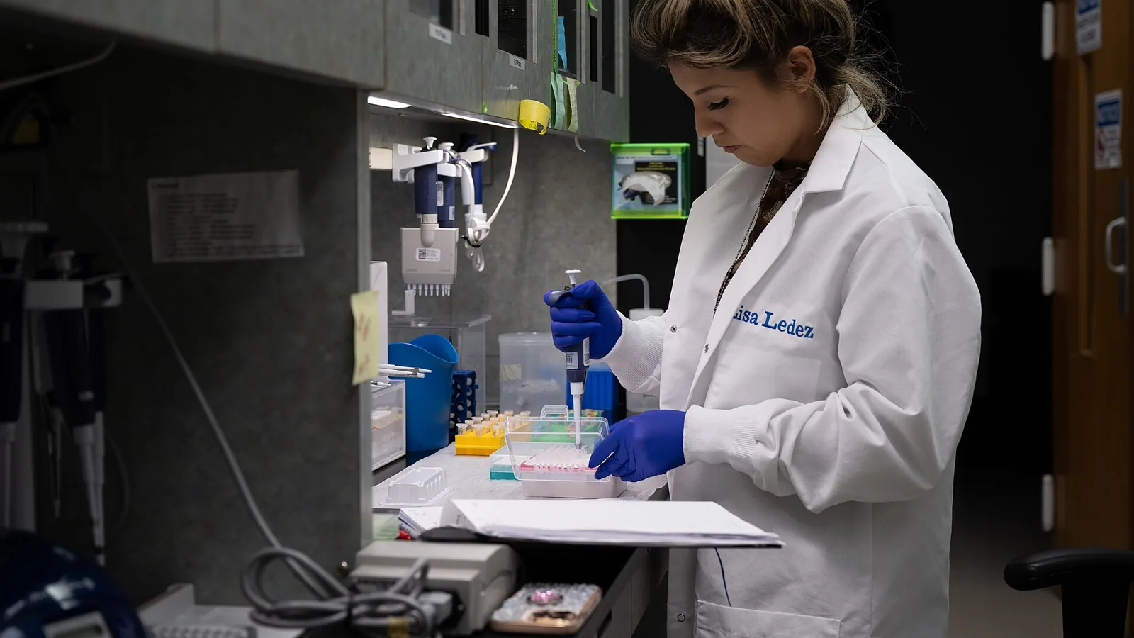
The Heartbreak of Failed qPCR: Your Guide to Perfect Efficiency
You're staring at your qPCR results at 2 AM, coffee cold beside you, seeing inconsistent Cq values that make no sense. That sinking feeling when your carefully planned experiment seems ruined by mysterious efficiency problems - we've all been there. This guide will walk you through every step of calculating, interpreting, and troubleshooting qPCR efficiency like a seasoned molecular biologist.
At a Glance: qPCR Efficiency Essentials
graph TD
    A[Standard Curve] --> B[Slope Calculation]
    B --> C[Efficiency Formula]
    C --> D[90-110% Target]
    D --> E{Troubleshoot?}
    E -->|Low Efficiency| F[Inhibition/Primer Issues]
    E -->|High Efficiency| G[Primer-Dimers]
Quantitative PCR (qPCR) efficiency is a measure of how effectively a target nucleic acid sequence is amplified during each cycle of the polymerase chain reaction. It is calculated from the slope of a standard curve generated by amplifying serial dilutions of a known template. The formula is: Efficiency (E) = 10^(-1/slope) - 1, where a perfect reaction yields an efficiency of 1.0 (or 100%). This calculation is essential for validating that your qPCR assay is performing optimally, ensuring accurate quantification of target DNA or RNA in your samples. It is most useful when setting up a new assay, comparing different primer sets, or troubleshooting inconsistent results.
At a Glance
| Aspect | Key Information |
|---|---|
| Purpose | Quantify amplification performance per cycle |
| Calculation | E = 10^(-1/slope) - 1, derived from standard curve slope |
| Ideal Efficiency | 1.0 (100%), meaning template doubles each cycle |
| Acceptable Range | 0.9–1.1 (90–110%) for most applications |
| Standard Curve | Minimum 5 dilution points, spanning 4–6 logs |
| Key Controls | No-template control (NTC), positive control, replicate consistency |
| Common Issues | Inhibition, poor primer design, pipetting errors, instrument variability |
Key Takeaways
- Quantitative PCR amplification efficiency (E) is calculated from the slope of a serial dilution standard curve using the equation: E = 10^(-1/slope) - 1 (or E% = [10^(-1/slope) - 1] × 100).
- An ideal qPCR assay demonstrates a standard curve slope of -3.322, reflecting 100% efficiency where the amplicon quantity doubles (2.0-fold) with every single thermal cycle.
- Acceptable clinical and MIQE guidelines require reaction efficiencies between 90% and 110% (slopes between -3.58 and -3.10) with an assay linearity correlation coefficient R² ≥ 0.98.
- Efficiencies exceeding 110% (slopes flatter than -3.10) indicate the presence of co-extracted PCR inhibitors (e.g., humic acid, ethanol, heme) in high-concentration standard points that dilute out at lower concentrations.
- Efficiencies below 90% point to suboptimal primer/probe annealing temperatures, secondary hairpin structures, depleted reagent master mixes, or non-specific primer-dimer competition.
Scientific Principle of qPCR Efficiency
qPCR relies on the exponential amplification of a target DNA sequence. During each cycle, the amount of target ideally doubles, producing a fluorescence signal proportional to the accumulating amplicon. The efficiency of this process determines how closely the reaction approaches the theoretical doubling. The standard curve method, described by Ruijter and van den Hoff (2025) [<a href="#ref-1">1</a>], uses a series of known template concentrations to establish the relationship between the quantification cycle (Cq) and the log of the initial template amount. The slope of this linear relationship directly reflects the amplification efficiency: a slope of -3.32 corresponds to 100% efficiency, while shallower slopes (less negative) indicate lower efficiency.
The mathematical foundation is straightforward. During exponential amplification, the amount of product after n cycles is given by: N = N0 × (1 + E)^n, where N0 is the initial template copy number and E is the efficiency. Taking the logarithm and rearranging yields the linear relationship between Cq and log(N0). The slope of this line is -1/log(1+E), which rearranges to the efficiency formula above. This principle is independent of the specific detection chemistry (SYBR Green, TaqMan probes, etc.) and applies to both absolute and relative quantification approaches.
Materials and Instrumentation Choices
Template Preparation
The quality of your standard curve depends critically on the template used. For absolute quantification, you need a well-characterized standard, such as a purified PCR product, plasmid DNA, or synthetic oligonucleotide. The template must be accurately quantified using an independent method (e.g., spectrophotometry, fluorometry, or digital PCR). For relative quantification, a validated reference sample or a dilution series of a pooled experimental sample can suffice, though absolute efficiency values may be less precise.
Dilution Series
Prepare serial dilutions in a consistent buffer (e.g., TE buffer or nuclease-free water with carrier RNA) to minimize adsorption losses at low concentrations. Use a minimum of five dilution points, ideally spanning 4–6 orders of magnitude. For example, a 10-fold dilution series from 10^6 to 10^1 copies/μL provides robust data. Each dilution should be prepared fresh and kept on ice to prevent degradation.
qPCR Master Mix
Choose a master mix appropriate for your detection chemistry and instrument. Commercial master mixes contain DNA polymerase, dNTPs, buffer, and fluorescent dye (e.g., SYBR Green) or probe components. The choice of polymerase affects efficiency: some enzymes have higher processivity or tolerance to inhibitors. Always use the same master mix batch for the entire experiment to avoid variability.
Instrument Calibration
Ensure your qPCR instrument is properly calibrated for the fluorescent dye you are using. Most modern instruments have automatic calibration, but periodic validation using manufacturer-provided calibration standards is recommended. The instrument's optical system and thermal uniformity directly impact the precision of Cq values and, consequently, efficiency calculations.
Controls and Their Importance
No-Template Control (NTC)
The NTC contains all reaction components except template. It detects contamination of reagents or consumables with target DNA. An NTC that produces a Cq value within 5 cycles of your lowest standard indicates significant contamination, which will distort efficiency calculations. For detailed guidance on NTC setup and interpretation, see the related article on No Template Control in qPCR.
Positive Control
Use a known positive sample (e.g., a purified plasmid at a defined concentration) to verify that the assay works as expected. The positive control should fall within the linear range of your standard curve. If its Cq deviates from the expected value by more than 0.5 cycles, investigate potential issues with template integrity or pipetting accuracy.
Replicate Consistency
Run each standard dilution and sample in at least triplicate. The coefficient of variation (CV) of Cq values within replicates should be less than 2% for reliable efficiency calculations. Higher variability suggests pipetting errors, template degradation, or instrument issues. Replicate outliers should be identified and excluded based on pre-defined criteria (e.g., Grubbs' test or a fixed threshold of ±0.5 cycles from the mean).
Negative Extraction Control
If you are extracting nucleic acids from samples, include a negative extraction control (e.g., nuclease-free water processed through the entire extraction protocol). This control identifies contamination introduced during extraction, which could affect efficiency calculations if the contaminant amplifies with the same primers.
Conceptual Workflow for Efficiency Calculation
Step 1: Prepare the Standard Curve
Create a serial dilution of your quantified template. For a 10-fold dilution series, mix 10 μL of the highest concentration with 90 μL of diluent, vortex thoroughly, and repeat for subsequent dilutions. Use a fresh pipette tip for each dilution to avoid carryover. The number of dilution points should be at least five, with the lowest concentration producing a Cq value within the detection limit of your assay (typically Cq < 35 for most instruments).
Step 2: Run the qPCR
Set up reactions according to your master mix manufacturer's instructions. Typical reaction volumes range from 10–25 μL. Include all standards, controls, and samples in the same plate to minimize inter-run variability. Use the same thermal cycling conditions for all reactions. The annealing temperature should be optimized for your primer set, typically 3–5°C below the calculated Tm of the primers.
Step 3: Analyze the Data
After the run, export the Cq values for each standard dilution. Plot Cq on the y-axis against log10 of the initial template concentration on the x-axis. Perform linear regression to obtain the slope and R² value. The slope should be negative, typically between -3.0 and -3.9. The R² value indicates the linearity of the standard curve; values above 0.99 are desirable.
Step 4: Calculate Efficiency
Apply the formula: Efficiency (E) = 10^(-1/slope) - 1. For example, if the slope is -3.32, then E = 10^(-1/-3.32) - 1 = 10^(0.301) - 1 = 2.00 - 1 = 1.00 (100%). If the slope is -3.50, then E = 10^(-1/-3.50) - 1 = 10^(0.286) - 1 = 1.93 - 1 = 0.93 (93%). Some software reports efficiency as a percentage (e.g., 93%) or as a factor (e.g., 1.93). Both are valid, but ensure consistency when comparing results.
Quality Checks for Standard Curves
Linearity (R²)
The coefficient of determination (R²) measures how well the data points fit the regression line. An R² value of 0.99 or higher indicates a strong linear relationship. Lower values suggest issues such as pipetting errors, template degradation, or non-specific amplification. If R² is below 0.98, repeat the standard curve with fresh dilutions.
Slope and Efficiency
The acceptable slope range for a 100% efficient reaction is -3.32 ± 0.1 (corresponding to 90–110% efficiency). Slopes shallower than -3.0 (efficiency > 120%) may indicate non-specific amplification or primer-dimer formation. Slopes steeper than -3.9 (efficiency < 80%) suggest inhibition or poor primer design. The efficiency value should be reported alongside the slope for clarity.
Dynamic Range
The standard curve should cover at least 4 orders of magnitude (e.g., 10^1 to 10^5 copies/μL). The linear range is the portion of the curve where the relationship between Cq and log concentration remains linear. If the highest or lowest dilutions deviate from linearity, they should be excluded from the regression. The dynamic range is the span of concentrations over which the assay can reliably quantify.
Reproducibility
Run the standard curve on at least two separate occasions to assess inter-run variability. The efficiency values should agree within 5% between runs. If not, investigate potential sources of variation such as reagent lot changes, instrument performance, or operator technique.
Interpreting Efficiency Results
Acceptable Efficiency Range
For most qPCR applications, an efficiency between 90% and 110% (0.9–1.1) is considered acceptable. This range accounts for minor variations in reaction conditions, pipetting accuracy, and instrument performance. Some stringent applications, such as clinical diagnostics or regulatory assays, may require efficiency between 95% and 105%. The acceptable range should be defined in your laboratory's standard operating procedures (SOPs).
Impact on Quantification
Efficiency directly affects the accuracy of quantification. If you assume 100% efficiency but the actual efficiency is 90%, the calculated target quantity will be underestimated by approximately 10% per cycle difference. For a 10-cycle difference in Cq, this error compounds to a 2.6-fold underestimation. Therefore, efficiency-corrected quantification methods, as described by Ruijter and van den Hoff (2025) [<a href="#ref-1">1</a>], are recommended for accurate results.
Efficiency and Relative Quantification
In relative quantification (e.g., the 2^(-ΔΔCq) method), equal amplification efficiencies of the target and reference genes are assumed. If efficiencies differ by more than 5%, the relative expression ratio will be biased. In such cases, use efficiency-corrected methods or optimize the assays to achieve comparable efficiencies.
Troubleshooting Poor Efficiency
Common Causes and Solutions
| Observation | Likely Cause | Discriminating Check |
|---|---|---|
| Efficiency > 110% | Non-specific amplification (primer-dimer) | Run melt curve analysis (SYBR Green) or gel electrophoresis; check for multiple peaks or bands |
| Efficiency > 110% | Pipetting errors in dilution series | Repeat the standard curve with fresh dilutions; verify pipette calibration |
| Efficiency < 90% | Inhibition from sample matrix | Dilute the sample 1:10 or 1:100; add internal positive control to test for inhibition |
| Efficiency < 90% | Poor primer design (secondary structure, low Tm) | Redesign primers using updated software; check for GC content and self-complementarity |
| Efficiency < 90% | Template degradation | Verify template integrity by gel electrophoresis or spectrophotometry; use fresh aliquots |
| Poor linearity (R² < 0.98) | Inconsistent pipetting | Use calibrated pipettes; pre-wet tips; vortex dilutions thoroughly |
| Poor linearity (R² < 0.98) | Template adsorption to tube walls | Use low-binding tubes; add carrier RNA (10 ng/μL) to diluent |
| High replicate variability | Instrument thermal non-uniformity | Run a plate uniformity test; ensure proper plate sealing |
| High replicate variability | Evaporation during cycling | Use optical adhesive film; ensure proper sealing |
Systematic Troubleshooting Approach
- Verify the standard curve: Prepare a fresh dilution series from a newly quantified stock. Run the curve in triplicate with a new master mix lot.
- Check primer specificity: Perform a BLAST search against the target genome. Run a no-template control and melt curve analysis to detect non-specific products.
- Test for inhibition: Spike a known amount of template into your sample and compare the Cq to the same amount in water. A delay of >1 cycle indicates inhibition.
- Optimize reaction conditions: Adjust annealing temperature (typically 55–65°C), primer concentration (100–500 nM each), or Mg²⁺ concentration (1.5–3.0 mM).
- Evaluate instrument performance: Run a calibration plate provided by the manufacturer. Check for consistent thermal cycling across the block.
Limitations of the Standard Curve Method
Assumption of Constant Efficiency
The standard curve method assumes that amplification efficiency is constant across all template concentrations and throughout the reaction. In reality, efficiency may decrease at very low template concentrations (due to stochastic effects) or at high concentrations (due to reagent depletion). This assumption is generally valid within the linear range of the curve but may break down at the extremes.
Dependence on Accurate Standard Quantification
The accuracy of the efficiency calculation depends on the accuracy of the standard's concentration. If the standard is misquantified by even 20%, the efficiency value will be biased. Independent quantification methods (e.g., digital PCR, spectrophotometry, or fluorometry) should be used to validate the standard concentration.
Sensitivity to Reaction Conditions
Efficiency can vary with changes in master mix composition, thermal cycling parameters, or instrument type. Therefore, efficiency should be recalculated whenever any component of the assay is changed. Inter-laboratory comparisons of efficiency values are only valid if the same reagents and protocols are used.
Not a Substitute for Validation
A good efficiency value does not guarantee that the assay is specific or accurate. Additional validation steps, such as sequencing of amplicons, specificity testing against related targets, and assessment of dynamic range, are necessary for a fully validated assay.
Documentation and Reporting
Essential Information to Record
- Date of experiment and operator name
- Template type and quantification method
- Dilution series scheme (concentrations and dilution factor)
- Master mix brand, lot number, and expiration date
- Thermal cycling conditions (annealing temperature, cycle numbers)
- Instrument model and software version
- Raw Cq values for all standards, controls, and samples
- Calculated slope, R², and efficiency
- Any deviations from the standard protocol
Reporting Standards
Follow the MIQE (Minimum Information for Publication of Quantitative Real-Time PCR Experiments) guidelines when reporting qPCR results. Include the efficiency value, slope, R², and dynamic range for each target. Report the method used for efficiency calculation (e.g., standard curve slope or amplification curve analysis). For absolute quantification, report the standard curve equation and the range of quantification.
Biosafety Considerations
BSL-1 Routine Practices
This article covers qPCR efficiency calculation using purified nucleic acids, which falls under BSL-1 containment. Standard microbiological practices apply: work in a clean, uncluttered area; wear lab coats and gloves; decontaminate work surfaces before and after experiments; and dispose of all waste according to institutional guidelines. The CDC and NIH BMBL (6th Edition) [<a href="#ref-2">2</a>] provides comprehensive guidance for BSL-1 practices.
Nucleic Acid Handling
Purified DNA or RNA is generally considered non-infectious, but it may be derived from organisms that require higher containment. Always follow institutional biosafety committee (IBC) approvals for the source material. The NIH Guidelines for Research Involving Recombinant or Synthetic Nucleic Acid Molecules [<a href="#ref-3">3</a>] provide a framework for risk assessment and containment of recombinant nucleic acids.
Decontamination
Use 10% bleach (0.5% sodium hypochlorite) or commercial DNA decontamination solutions to clean work surfaces and equipment. UV irradiation can also reduce DNA contamination but may not be sufficient for complete decontamination. Ensure that all pipettes, tube racks, and instruments are decontaminated regularly.
Preventing Contamination
Use dedicated pipettes and filter tips for qPCR setup. Prepare master mixes in a separate area from template addition. Use positive displacement pipettes for viscous solutions. Include no-template controls in every run to monitor for contamination.
Frequently Asked Questions
1. Can I calculate qPCR efficiency without a standard curve?
Yes, efficiency can also be estimated from the amplification curve itself using methods such as the "window-of-linearity" or "LinRegPCR" approach. These methods analyze the exponential phase of individual amplification curves to calculate efficiency per sample. However, the standard curve method remains the most widely accepted and straightforward approach for initial assay validation. The amplification curve method is more suitable for relative quantification when a standard curve is not available.
2. What should I do if my efficiency is consistently above 110%?
Efficiency above 110% often indicates non-specific amplification, such as primer-dimer formation or amplification of off-target sequences. Run a melt curve analysis (for SYBR Green assays) or gel electrophoresis to check for multiple products. If non-specific products are present, redesign primers or increase the annealing temperature. If no non-specific products are detected, check your dilution series for pipetting errors that might compress the Cq range.
3. How many dilution points do I need for a reliable efficiency calculation?
A minimum of five dilution points is recommended, with at least three replicates per point. Fewer points reduce the statistical power of the linear regression and may not adequately capture the dynamic range. For high-precision applications, use six to eight dilution points spanning 5–6 orders of magnitude. The lowest dilution should produce a Cq value at least 3 cycles above the no-template control.
4. Can I use the same standard curve for multiple experiments?
Standard curves should be generated fresh for each experiment if absolute quantification is required. For relative quantification, a validated standard curve can be reused if the assay conditions (master mix, primers, instrument) remain unchanged and the curve is re-evaluated periodically (e.g., every 3–6 months). However, any change in reagents or instrument requires a new standard curve. Inter-run variability should be monitored using a reference sample included in every run.
Related Clinical & Scientific Guides
- Loop-Mediated Isothermal Amplification (LAMP) Assay for Rapid Detection of African Swine Fever Virus in Oral Fluids
- How to Calculate the Concentration of Protein Using the Lowry Assay
- DNA Extraction from Saliva: Non-Invasive Sampling and Protocols
References and Further Reading
[1] Ruijter JM, van den Hoff MJB. Analysis of qPCR Data: From PCR Efficiency to Absolute Target Quantity. 2025. PubMed ID: 41465312. [Link](https://pubmed.ncbi.nlm.nih.gov/41465312/) [2] Provides an example of qPCR standard curve generation and validation for pathogen detection. [3] Arshinova ES, Karpova NS, Terekhina OL, et al. Improved Step-by-Step qPCR Method for Absolute Telomere Length Measurement. 2026. PubMed ID: 41718324. [Link](https://pubmed.ncbi.nlm.nih.gov/41718324/) [4] Describes the theoretical basis for efficiency-corrected [qPCR analysis](/knowledge/diagnostics/molecular/qpcr-analysis-plate-layout-delta-delta-ct) and methods for absolute quantification. [5] Pinheiro GL, Lin NJ, Parratt KH, et al. The Integration of Focused Ultrasonication, ddPCR, and Flow Cytometry Effectively Estimates Genome Copies per Cell and Enhances DNA Extraction Efficiency in Escherichia coli Samples. 2026. PubMed ID: 42077846. [Link](https://pubmed.ncbi.nlm.nih.gov/42077846/) [6] Discusses DNA extraction efficiency and its impact on qPCR quantification accuracy. [7] Zhu W, Zhu H. Development of a multiplex fluorescent qPCR assay for the simultaneous detection of [bovine viral diarrhea virus](/knowledge/viruses/livestock-viruses/bovine-viral-diarrhea-virus) and pathogenic Escherichia coli. 2026. PubMed ID: 42139222. [Link](https://pubmed.ncbi.nlm.nih.gov/42139222/) [8] Demonstrates standard curve methodology for absolute quantification using oligonucleotide standards. [9] Fu J, Yu L, Fu Z, et al. An Improved Method for Determining the Infection Titer of Replication-Competent Adeno-Associated Virus. 2026. PubMed ID: 41898299. [Link](https://pubmed.ncbi.nlm.nih.gov/41898299/) [10] Illustrates standard curve preparation and quality metrics (linearity, sensitivity, reproducibility) for qPCR-based titer determination. [11] CDC and NIH. Biosafety in Microbiological and Biomedical Laboratories (BMBL), 6th Edition. 2020. [Link](https://www.cdc.gov/labs/bmbl/index.html) [12] Authoritative guidance on biosafety practices for laboratory work with nucleic acids. [13] National Institutes of Health. NIH Guidelines for Research Involving Recombinant or Synthetic Nucleic Acid Molecules. [Link](https://osp.od.nih.gov/policies/biosafety-and-biosecurity-policy/nih-guidelines-for-research-involving-recombinant-or-synthetic-nucleic-acid-molecules/) [14] Framework for risk assessment and containment of recombinant nucleic acid research. [15] National Center for Biotechnology Information. NCBI Bookshelf: Molecular Biology and Laboratory Methods. [Link](https://www.ncbi.nlm.nih.gov/books/) [16] Searchable collection of authoritative methods references for molecular biology techniques.Related Articles
- How to Calculate PCR Efficiency from a Standard Curve
- qPCR Efficiency: Why It Matters and How to Improve It
- No Template Control (NTC) in qPCR: Setup, Interpretation, and Troubleshooting
- Understanding qPCR Amplification Curves: Shape, Threshold, and Interpretation
- How to Calculate and Interpret qPCR Efficiency from a Standard Curve
- Absolute Quantification Using qPCR: Standard Curves and Copy Number Calculation
Frequently Asked Questions (Structured PCR Efficiency FAQ)
Q1: What is the acceptable qPCR efficiency range?
Answer: Optimal efficiency is $90\%\text{ to }110\%$ (corresponding to standard curve slopes between $-3.58\text{ and }-3.10$ with $R^2 > 0.985$).
Q2: What causes qPCR efficiency below $90\%$?
Answer: Slopes steeper than $-3.58$ indicate poor primer binding, sub-optimal annealing temperatures, suboptimal magnesium ($ ext{Mg}^{2+}$) concentration, or degraded reagents.
Q3: How do PCR inhibitors affect standard curve slopes?
Answer: Inhibitors disproportionately suppress amplification in concentrated standard samples, making the high-concentration Ct values appear abnormally late and artificially flattening the curve (yielding false $>110\%$ efficiency).