How to Calculate the Number of Bacteria in a Sample Using Direct Microscopic Count
By Dr. Zubair Khalid, DVM, MS, PhD ·
Key Takeaways
- Direct microscopic count, also known as the Breed count, provides a rapid, culture-independent estimation of total bacterial cells (viable and non-viable) in a liquid sample within 20-40 minutes.
- The method relies on enumerating cells within a precisely defined volume using a calibrated counting chamber (e.g., Petroff-Hausser or hemocytometer) and a microscope with a calibrated eyepiece graticule.
- A critical limitation is the inability to distinguish between live and dead cells without the use of specific viability stains (e.g., LIVE/DEAD BacLight kit) and fluorescence microscopy.
- The practical detection limit is approximately 10⁶ cells/mL; lower concentrations require sample concentration methods like centrifugation or membrane filtration for reliable enumeration.
- Accurate calculation requires careful sample preparation (including appropriate dilutions), systematic counting with defined inclusion/exclusion criteria, and application of volume and dilution correction factors.
- Quality control measures such as replicate counts, uniformity assessment (CV calculation), and comparison with independent methods (e.g., plate counts) are essential for validating results.
The direct microscopic count method, also known as the Breed count method, estimates the total number of bacterial cells in a liquid sample by directly visualizing and enumerating cells under a microscope. This technique provides a rapid, culture-independent measurement of total cell count, including both viable and non-viable cells, within approximately 30 minutes. It is most useful when you need immediate estimates of bacterial abundance, when working with samples containing slow-growing or non-culturable organisms, or when validating other enumeration methods such as plate counts or flow cytometry. The calculation converts the average number of cells observed per microscope field into cells per milliliter of original sample using known geometric factors of the counting chamber and microscope setup.
At a Glance
| Aspect | Detail |
|---|---|
| Method type | Direct, culture-independent total cell count |
| Time required | 20–40 minutes (sample preparation through calculation) |
| Equipment needed | Compound microscope with calibrated stage micrometer, counting chamber (hemocytometer or Petroff-Hausser), pipettes, coverslip |
| Output | Total cells per milliliter (cells/mL) |
| Distinguishes live/dead? | No, unless combined with viability stains |
| Detection limit | Approximately 10⁶ cells/mL for reliable counting |
| Best for | Concentrated bacterial suspensions, environmental samples, quality control of starter cultures |
| Key limitation | Cannot distinguish viable from non-viable cells without special staining |
Scientific Principle
Direct microscopic counting relies on the relationship between the volume of sample examined and the number of cells observed within a defined area. A counting chamber, typically a hemocytometer for eukaryotic cells or a Petroff-Hausser chamber for bacteria, contains a grid of known dimensions etched onto a glass surface. When a coverslip is placed over the chamber, a precise depth (usually 0.02 mm for bacterial counting) is established. The volume above each grid square is therefore fixed and calculable.
The fundamental equation is:
Cells per mL = (Average cells per grid square) × (Dilution factor) × (Volume correction factor)
The volume correction factor converts the volume of one grid square to 1 mL. For a Petroff-Hausser chamber with a depth of 0.02 mm and a grid square area of 0.0025 mm² (50 µm × 50 µm), the volume per square is 5 × 10⁻⁸ mL. The correction factor is therefore 1 / (5 × 10⁻⁸) = 2 × 10⁷.
This approach assumes that cells are uniformly distributed throughout the sample and that the counted fields are representative of the entire suspension. The method counts all particles that appear bacterial in morphology, which is why it provides a total cell count rather than a viable count [<a href="#ref-1">1</a>]. As noted in the MATRIX workflow, direct microscopic counting remains low-throughput and prone to user variability, but it provides essential quantitative data that indirect methods like optical density cannot match [<a href="#ref-1">1</a>].
Materials and Instrumentation Choices
Microscope Requirements
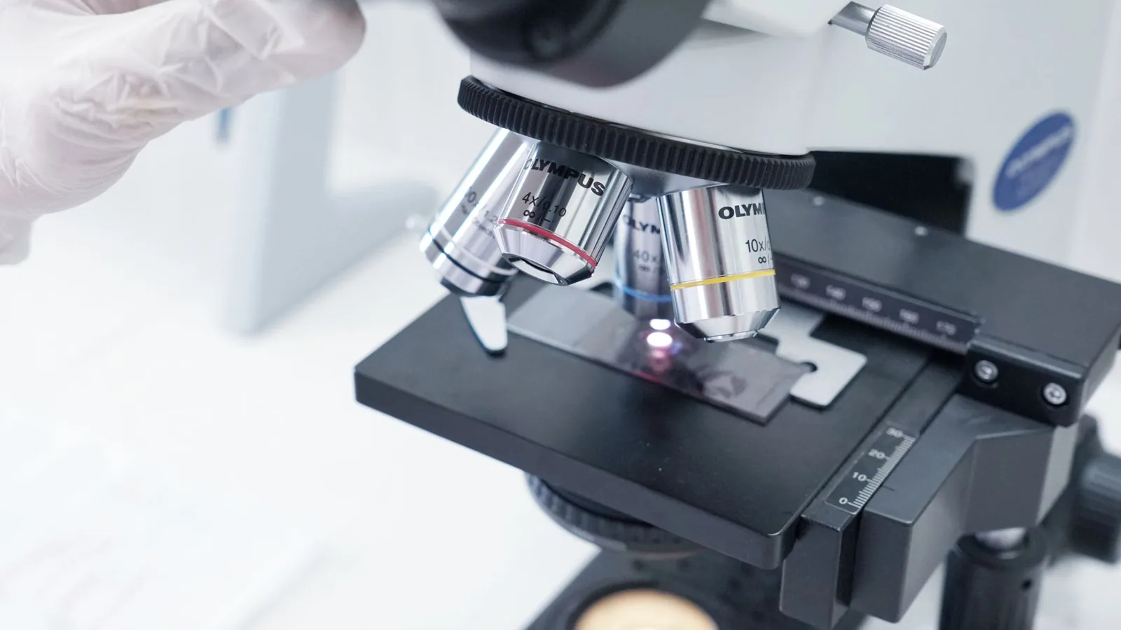
A standard compound light microscope with phase-contrast capability is strongly recommended for bacterial counting. Bright-field microscopy can be used if cells are stained, but phase-contrast allows visualization of unstained cells by enhancing contrast based on refractive index differences. The microscope must have:
- 40× objective (minimum) for bacterial visualization; 100× oil immersion is preferred for small cells (0.5–2 µm)
- 10× eyepieces with a calibrated eyepiece graticule
- Mechanical stage for systematic field selection
Counting Chamber Selection
Two primary chamber types exist for bacterial counting:
Petroff-Hausser counting chamber: Designed specifically for bacteria, with a depth of 0.02 mm and grid squares of 0.0025 mm². The chamber holds approximately 0.02 mL total volume. This is the preferred choice for bacterial suspensions because the shallow depth keeps bacteria in a single focal plane.
Hemocytometer: Originally designed for blood cell counting, with a depth of 0.1 mm and larger grid squares (0.04 mm²). While usable for bacteria, the greater depth means cells may settle at different focal planes, requiring careful focusing. The volume per large square is 0.004 mL, giving a correction factor of 250.
Your choice depends on expected cell concentration. The Petroff-Hausser chamber accommodates higher cell densities (10⁶–10⁹ cells/mL) without requiring dilution, while the hemocytometer is better suited for lower concentrations or when counting larger bacterial cells.
Stains and Reagents
For bright-field counting, a simple stain is necessary:
- Methylene blue (0.1% w/v): Stains cells blue against a light background. Does not distinguish live from dead.
- Gram stain: Can be used but adds complexity and may cause cell clumping.
- Acridine orange: Fluorescent stain that binds nucleic acids; requires fluorescence microscopy but allows differentiation of metabolically active cells when used with appropriate filters [<a href="#ref-1">1</a>].
For viability assessment, combine with:
- LIVE/DEAD BacLight kit: Uses SYTO 9 (green, all cells) and propidium iodide (red, membrane-compromised cells). Requires fluorescence microscopy.
Calibration Tools
- Stage micrometer: A slide with an engraved scale (typically 1 mm divided into 100 divisions of 0.01 mm each). Used to calibrate the eyepiece graticule.
- Eyepiece graticule: A glass disc with a ruled scale that fits inside the eyepiece. Must be calibrated against the stage micrometer for each objective lens used.
Controls and Standards
Positive Control
Prepare a standardized bacterial suspension of known concentration (e.g., Escherichia coli K-12 at approximately 10⁸ cells/mL, verified by plate count). Count this suspension using your direct microscopic method. The result should fall within 20% of the expected value. If it does not, check your calibration, chamber loading technique, and counting criteria.
Negative Control
Count the sterile diluent (e.g., phosphate-buffered saline, 0.85% saline) alone. This should yield zero bacterial cells per field. Any observed particles indicate contamination of reagents or the counting chamber.
Replicate Counts
Count at least three separate chamber loadings from the same sample. For each loading, count a minimum of 10 fields (for Petroff-Hausser) or 5 large squares (for hemocytometer). Calculate the mean and standard deviation. A coefficient of variation (CV) exceeding 30% suggests uneven cell distribution or counting errors.
Instrument Calibration
Before each counting session, verify the eyepiece graticule calibration using the stage micrometer. Record the calibration factor for each objective lens. For phase-contrast microscopy, ensure proper alignment of phase rings according to the manufacturer's instructions.
Conceptual Workflow
Step 1: Sample Preparation
If the sample is too concentrated (more than approximately 20 cells per small grid square), prepare a serial dilution in sterile buffer. The goal is to achieve 5–15 cells per counting square for optimal accuracy. Record all dilution factors precisely.
For environmental samples containing particulate matter (soil, sediment, biofilm), you may need to disperse cells before counting. Add 0.1% sodium pyrophosphate and vortex for 30 seconds, or sonicate briefly (30 seconds at low power) to break up clumps without lysing cells [<a href="#ref-1">1</a>].
Step 2: Chamber Loading
Clean the counting chamber and coverslip with 70% ethanol and allow to air dry. Moisten the coverslip slightly and press it onto the chamber until Newton's rings (rainbow interference patterns) appear, indicating proper seating. Pipette 10–20 µL of well-mixed sample at the edge of the coverslip. Capillary action will draw the sample into the chamber. Do not overfill or allow bubbles to form.
Step 3: Microscopic Examination
Allow the chamber to sit undisturbed for 2–3 minutes to let cells settle onto the grid surface. Focus on the grid using the 10× objective, then switch to 40× or 100× oil immersion. For phase-contrast, adjust the phase ring alignment.
Systematically count cells in at least 10 grid squares for a Petroff-Hausser chamber, or 5 large squares for a hemocytometer. Use a hand tally counter to track counts. Establish clear inclusion/exclusion criteria:
- Count cells that touch the top and left borders of each square
- Do not count cells touching the bottom and right borders (to avoid double-counting)
- Count clumps as individual cells only if you can distinguish separate cell boundaries; otherwise, count the clump as one "colony-forming unit" equivalent
Step 4: Calculate Average Cells per Square
Sum the counts from all squares and divide by the number of squares counted. For example, if you counted 10 squares with totals of 8, 12, 7, 9, 11, 6, 10, 8, 13, and 9 cells, the sum is 93, and the average is 9.3 cells per square.
Step 5: Apply Volume Correction Factor
For a Petroff-Hausser chamber (depth 0.02 mm, square area 0.0025 mm²):
- Volume per square = 0.02 mm × 0.0025 mm² = 5 × 10⁻⁵ mm³ = 5 × 10⁻⁸ mL
- Correction factor = 1 / (5 × 10⁻⁸) = 2 × 10⁷
For a hemocytometer (depth 0.1 mm, large square area 0.04 mm²):
- Volume per large square = 0.1 mm × 0.04 mm² = 0.004 mm³ = 4 × 10⁻⁶ mL
- Correction factor = 1 / (4 × 10⁻⁶) = 2.5 × 10⁵
Step 6: Apply Dilution Factor
Multiply the result from Step 5 by the dilution factor. If you diluted the sample 1:10 (10-fold), the dilution factor is 10.
Step 7: Final Calculation
Cells per mL = (Average cells per square) × (Correction factor) × (Dilution factor)
Example: Average 9.3 cells/square, Petroff-Hausser chamber, 1:10 dilution = 9.3 × 2 × 10⁷ × 10 = 1.86 × 10⁹ cells/mL
Quality Checks
Uniformity Assessment
Calculate the coefficient of variation (CV) across your counted fields: CV (%) = (Standard deviation / Mean) × 100
A CV below 20% indicates acceptable uniformity. Higher values suggest:
- Incomplete mixing before chamber loading
- Cell clumping
- Counting errors (inconsistent inclusion/exclusion criteria)
- Uneven chamber filling
Linearity Check
If you counted multiple dilutions, plot log(cells/mL) versus log(dilution factor). The relationship should be linear with a slope of approximately -1. Deviations indicate counting artifacts at high or low concentrations.
Comparison with Independent Method
Whenever possible, compare your direct microscopic count with a plate count (viable count) from the same sample. The direct count should be higher than the viable count because it includes dead and dormant cells. A ratio of direct count to viable count (D/V ratio) between 2 and 10 is typical for healthy bacterial cultures. Ratios exceeding 100 suggest a large proportion of dead or non-culturable cells, which may be expected in environmental samples [<a href="#ref-1">1</a>].
Troubleshooting
| Observation | Likely Cause | Discriminating Check |
|---|---|---|
| Cells appear blurry or out of focus | Incorrect focal plane; chamber depth too great for objective | Use phase-contrast; switch to 40× objective; ensure coverslip is properly seated |
| Uneven cell distribution across fields | Incomplete mixing; chamber not level | Vortex sample for 30 seconds; re-level microscope stage; count additional fields |
| Bubbles in counting chamber | Air trapped during loading | Clean chamber and reload; ensure coverslip is moistened evenly |
| Cells moving during counting | Brownian motion; chamber not settled | Wait 3–5 minutes before counting; fix sample with 0.5% formalin if necessary |
| Counts decrease over time | Cells settling in pipette tip | Vortex sample between chamber loadings; work quickly |
| Particulate debris mistaken for cells | Sample contains non-cellular particles | Stain with methylene blue; use phase-contrast to distinguish refractive bacteria from debris |
| Very low counts (<1 cell per square) | Sample too dilute | Concentrate by centrifugation (10,000 × g, 10 min) and resuspend in smaller volume; or switch to membrane filtration method |
| Very high counts (>50 cells per square) | Sample too concentrated | Prepare additional dilutions; count smaller grid squares if available |
| Inconsistent counts between replicate loadings | Pipetting error; chamber contamination | Use calibrated pipette; clean chamber between loadings; prepare fresh dilutions |
Limitations and Considerations
Inability to Distinguish Viable from Non-Viable Cells
Standard direct microscopic counting provides total cell count, not viable count. This is a critical distinction when assessing the effectiveness of antimicrobial treatments or pasteurization processes. For example, a study on nanosecond pulsed electric field treatment of human milk reported that microscopic analysis revealed residual bacterial counts of 2–3 log CFU/mL post-treatment, but these counts represented both viable and non-viable cells [<a href="#ref-2">2</a>]. To assess viability, you must combine direct counting with viability stains such as the LIVE/DEAD BacLight kit or with metabolic activity indicators like CTC (5-cyano-2,3-ditolyl tetrazolium chloride) [<a href="#ref-1">1</a>].
Detection Limit
The practical detection limit for direct microscopic counting is approximately 10⁶ cells/mL. Below this concentration, the statistical uncertainty becomes unacceptably high because you would need to count hundreds of fields to obtain reliable estimates. For samples with lower bacterial concentrations, consider membrane filtration followed by direct staining on the filter, or use flow cytometry [<a href="#ref-3">3</a>].
User Variability
Direct counting is operator-dependent. Different users may apply different inclusion/exclusion criteria, focus differently, or fatigue over time. The MATRIX workflow addresses this by integrating automated microscopy and image analysis, which reduces user variability and increases throughput [<a href="#ref-1">1</a>]. For manual counting, train all operators using the same reference images and perform regular inter-operator comparison exercises.
Cell Clumping
Bacteria that naturally form chains (e.g., Streptococcus spp.) or clumps (e.g., Staphylococcus spp.) present a challenge. Standard practice is to count each visible cell individually if boundaries are distinguishable. If clumps are too dense to resolve, report results as "clump-forming units" and note the limitation. Sonication or vortexing with glass beads can help disperse clumps, but may also lyse some cells.
Sample Matrix Interference
Complex samples such as soil suspensions, milk, or biofilm homogenates contain particles that can be mistaken for bacteria. The study on microplastic detection noted that environmental matrices present significant challenges for optical methods due to chemical diversity and complexity [<a href="#ref-3">3</a>]. For such samples, use specific fluorescent stains (e.g., DAPI for DNA, SYTO 9 for nucleic acids) and appropriate filter sets to distinguish bacteria from abiotic particles.
Documentation and Reporting
Essential Data to Record
For each counting session, document:
- Sample identification and source
- Date and time of collection and counting
- Operator name
- Counting chamber type and manufacturer
- Microscope model, objectives used, and calibration factor
- Stain used (if any)
- Number of fields counted
- Individual field counts
- Mean, standard deviation, and CV
- Dilution factor(s)
- Final calculated concentration (cells/mL)
- Any observations (clumping, debris, unusual morphology)
Reporting Format
Report results as: X.XX × 10^Y cells/mL (direct microscopic count, Petroff-Hausser chamber, n=10 fields, CV=XX%)
Include the 95% confidence interval: Mean ± (1.96 × SEM), where SEM = standard deviation / √(number of fields).
Quality Documentation
Maintain a log of:
- Chamber calibration dates and results
- Positive and negative control results
- Inter-operator comparison results
- Any deviations from standard protocol
Biosafety Considerations
Risk Assessment
Direct microscopic counting of known, non-pathogenic bacteria (Biosafety Level 1) can be performed on an open bench with standard microbiological practices. However, you must still follow the principles outlined in the Biosafety in Microbiological and Biomedical Laboratories (BMBL) 6th Edition [<a href="#ref-4">4</a>]:
- Wear a laboratory coat and gloves
- Work on a disinfected surface
- Decontaminate the counting chamber and coverslip with 70% ethanol or 10% bleach after use
- Dispose of contaminated pipette tips and slides in biohazard waste
Sample Handling
If the sample origin is unknown or potentially contains pathogens, treat it as BSL-2 until characterized. For environmental samples, assume the presence of opportunistic pathogens and use appropriate containment. The NIH Guidelines for Research Involving Recombinant or Synthetic Nucleic Acid Molecules provide additional framework if you are working with genetically modified organisms [<a href="#ref-5">5</a>].
Decontamination Protocol
After counting:
- Disassemble the counting chamber and separate the coverslip
- Immerse both in 10% bleach solution for 30 minutes
- Rinse thoroughly with distilled water
- Air dry and store in a clean, dust-free container
- Wipe down the microscope stage and objectives with 70% ethanol
Spill Management
If a sample spills on the microscope or bench:
- Cover the spill with absorbent paper
- Apply 10% bleach solution from the edges inward
- Allow 20 minutes contact time
- Wipe up and dispose of paper in biohazard waste
- Disinfect the area again with 70% ethanol
Frequently Asked Questions
Q1: Why is my direct microscopic count always higher than my plate count? This is expected and normal. Direct microscopic counting enumerates all cells present, including dead, dormant, and viable-but-non-culturable (VBNC) cells. Plate counts only detect cells capable of forming colonies under the specific growth conditions provided. The ratio of direct count to viable count (D/V ratio) provides information about the physiological state of the population. A ratio of 2–10 is typical for healthy cultures, while higher ratios indicate stress or environmental exposure.
Q2: How many fields should I count to get a reliable estimate? Count a minimum of 10 fields for a Petroff-Hausser chamber or 5 large squares for a hemocytometer. However, the optimal number depends on the variability between fields. Calculate the cumulative mean after each field; once the cumulative mean stabilizes (changes by less than 10% over 5 consecutive fields), you have counted enough fields. For samples with high variability (CV > 30%), count 20–30 fields to improve precision.
Q3: Can I use direct microscopic counting for environmental samples like soil or water? Yes, but with modifications. Soil samples require extensive dispersion and dilution to separate cells from particles. Water samples with low bacterial concentrations (<10⁶ cells/mL) need concentration by filtration or centrifugation. For both sample types, use fluorescent nucleic acid stains (DAPI, SYTO 9) and epifluorescence microscopy to distinguish bacteria from abiotic particles. The MATRIX workflow demonstrates that automated image analysis can improve reproducibility for environmental microbiomes [<a href="#ref-1">1</a>].
Q4: What is the smallest bacterium I can reliably count with this method? With a 100× oil immersion objective (total magnification 1000×), you can resolve bacteria as small as 0.2–0.3 µm, which covers most known bacteria. However, very small cells (e.g., Mycoplasma species at 0.1–0.3 µm) may be difficult to distinguish from debris. For such samples, use specific fluorescent probes targeting bacterial ribosomal RNA or DNA, and employ a high-resolution camera for image capture. Phase-contrast microscopy at 1000× magnification provides better contrast for small, unstained cells than bright-field microscopy.
Related Clinical & Scientific Guides
- Loop-Mediated Isothermal Amplification (LAMP) Assay for Rapid Detection of African Swine Fever Virus in Oral Fluids
- How to Calculate the Concentration of Protein Using the Lowry Assay
- DNA Extraction from Saliva: Non-Invasive Sampling and Protocols
References and Further Reading
[1] **MATRIX: Rapid Quantification of Total and Active Microbial Cells with Single-Cell Phenotypes for Environmental Microbiomes** – Gonzalo M, Liu X, Dufour YS, Shade A. (2026). *bioRxiv*. https://doi.org/10.64898/2026.03.16.712149 [2] **Evaluating continuous nanosecond pulsed electric field (nsPEF) treatment as a non-thermal alternative for human milk pasteurisation** – Wang Y, Zare F, Prabawati EK, et al. (2025). *PubMed*. https://pubmed.ncbi.nlm.nih.gov/41191605/ [3] **Optical, Chemical, and Biological Detection Methods of Microplastics and Nanoplastics** – Vico C, Chua SL. (2026). *PubMed*. https://pubmed.ncbi.nlm.nih.gov/42326851/ [4] **Biosafety in Microbiological and Biomedical Laboratories (BMBL), 6th Edition** – CDC and NIH. (2020). U.S. Department of Health and Human Services. https://www.cdc.gov/labs/bmbl/index.html [5] **NIH Guidelines for Research Involving Recombinant or Synthetic Nucleic Acid Molecules** – National Institutes of Health. https://osp.od.nih.gov/policies/biosafety-and-biosecurity-policy/nih-guidelines-for-research-involving-recombinant-or-synthetic-nucleic-acid-molecules/ [6] **NCBI Bookshelf: Molecular Biology and Laboratory Methods** – National Center for Biotechnology Information. https://www.ncbi.nlm.nih.gov/books/Searchable collection of authoritative methods references for additional protocols and background information.
Related Articles
- How to Calculate the Number of Bacteria in a Sample Using the Surface Spread Method
- How to Calculate the Number of Bacteria in a Sample Using Flow Cytometry
- How to Calculate the Number of Bacteria in a Sample Using ATP Bioluminescence
- How to Calculate the Number of Bacteria in a Sample Using the Pour Plate Method
- How to Calculate the Number of Bacteria in a Sample Using the Spread Plate Method
- How to Calculate the Number of Bacteria in a Sample Using the Membrane Filtration Method