CLSM Microscopy: Confocal Laser Scanning Basics
By Dr. Zubair Khalid, DVM, MS, PhD ·
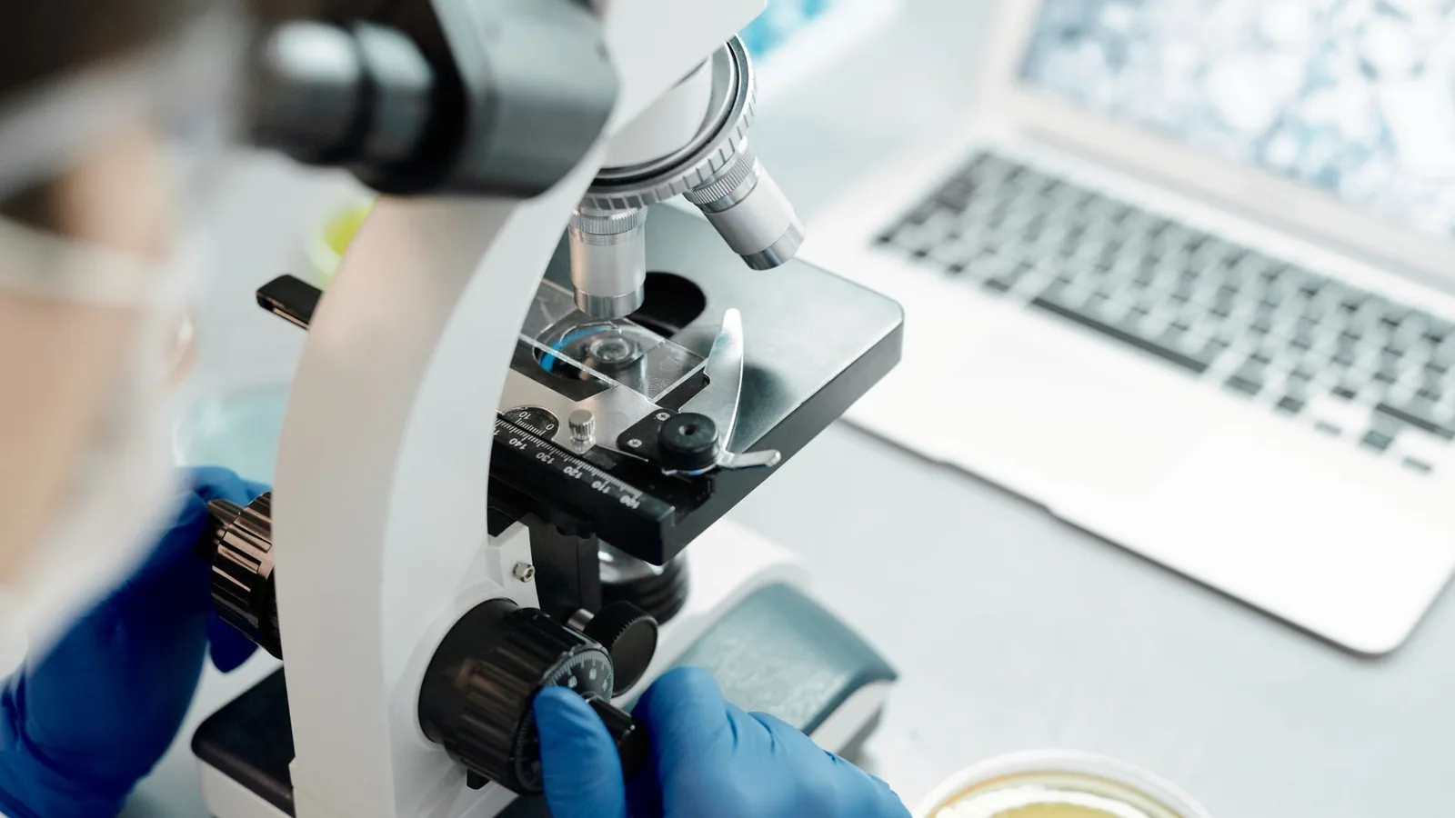
Confocal laser scanning microscopy (CLSM) is a fluorescence imaging method that uses a focused laser, a scanning mirror system, and a small aperture called a pinhole to collect light from one thin plane of a specimen at a time. The pinhole physically blocks emission from above and below the focal plane, so the instrument builds an optical section instead of a blurred full-thickness view.
That single design decision, rejecting out-of-focus light rather than physically cutting the sample, is why CLSM microscopy became the default tool for looking inside intact cells, thick tissue, biofilms, and mineralized structures such as dentin. A histology slide requires a microtome, dehydration, and sectioning that destroys three-dimensional context. A confocal microscope produces the same thin-plane view from a living or fixed specimen that stays whole, and it can repeat that view at many depths to reconstruct a volume [1].
What CLSM Actually Measures
CLSM detects fluorescence. A fluorophore absorbs photons at one wavelength band and re-emits them at a longer wavelength band. The microscope records the emitted photons, and pixel brightness maps to fluorophore concentration at that point in space. Everything else in the instrument exists to make sure the recorded photon came from the plane you selected.
This is different from reflectance confocal microscopy, which detects backscattered light rather than fluorescence and is used for near-histologic skin imaging, including monitoring treatment response in locally advanced basal cell carcinoma [2]. It is also different from line-field confocal optical coherence tomography, which combines vertical optical coherence tomography sections with confocal en face imaging and has been used to map epithelial stratification in lingual mucosa [3]. The confocal principle is shared. The contrast mechanism is not.
Why Optical Sectioning Matters
A widefield fluorescence microscope illuminates the whole depth of the specimen. Emission from every plane reaches the camera at once, and the resulting image is a superposition of sharp in-focus detail and a haze of out-of-focus blur. Deconvolution can partially correct this computationally, but it cannot recover information the optics never isolated.
Confocal sectioning is an optical, not physical, separation. The specimen is never sliced. This matters for two practical reasons. First, the sample survives, so the same region can be imaged repeatedly over time, which is the basis of live-cell confocal work. Second, depth information is preserved, so a stack of optical sections can be rendered as a three-dimensional volume, as demonstrated in large-area corneal reconstructions built from laterally extended in vivo confocal datasets [1].
The Light Path, Step by Step
- A laser emits a narrow band of light at the excitation wavelength of the chosen fluorophore.
- The beam passes through an excitation filter that removes plasma lines and off-band emission from the laser source.
- A dichroic mirror reflects the excitation light toward the specimen while transmitting longer-wavelength emission on the return path.
- An objective lens focuses the beam to a diffraction-limited spot inside the specimen.
- Fluorophores in that spot emit light at longer wavelengths.
- The same objective collects the emission and passes it back through the dichroic mirror.
- An emission filter removes any residual excitation light and restricts the detected band.
- The pinhole aperture sits at the image plane and passes light from the focal point while blocking light from other depths.
- A photomultiplier tube or similar detector converts the transmitted photons into an electrical signal.
- Galvanometer mirrors raster the beam across the field, building the image pixel by pixel.
The pinhole is the heart of the design. Its conjugate position relative to the focal spot means that a photon emitted from a plane 2 µm above focus converges at a different point and is largely stopped by the aperture edge.
Excitation and Emission Filter Selection
Filter choice determines which fluorophores you can separate and how much signal reaches the detector. Three components do the work.
The excitation filter narrows the laser output to the fluorophore absorption band. A 488 nm laser line excites fluorescein, GFP, and Alexa Fluor 488 efficiently. A 561 nm line excites rhodamine B, tetramethylrhodamine, and mCherry. A 640 nm line excites far-red dyes such as Alexa Fluor 647.
The dichroic mirror is a long-pass or multi-band reflector placed at 45 degrees. It reflects short-wavelength excitation toward the sample and transmits longer-wavelength emission toward the detector. Its cutoff must sit between the excitation and emission peaks of every fluorophore in the panel.
The emission filter is a band-pass element that defines the detection window. A typical setting for a red dye is 570 to 670 nm, which is the configuration validated for Nile Red-assisted confocal detection of airborne micro- and nanoplastics, where an optimized 561 nm excitation with 570 to 670 nm emission significantly improved particle recovery while keeping nonpolymeric particulates such as mineral particles and activated carbon from producing meaningful fluorescence interference [4]. That study also showed that a non-optimized fluorescence configuration can substantially underestimate particle abundance, especially below 1 µm, which is a direct demonstration of how much filter choice controls what you actually see.
Spectral Overlap and Compensation
When two fluorophores have overlapping emission spectra, some of the signal from one channel bleeds into the other. This is spectral crosstalk. It is corrected in three ways. Sequential line scanning excites one fluorophore at a time and collects only its emission before switching. Spectral unmixing uses reference spectra from single-stained controls to mathematically separate the contributions. Narrower emission bands reduce overlap at the cost of collected photons.
The practical rule is that any panel with more than two fluorophores needs single-stain controls and, ideally, an unstained control to measure autofluorescence. Without those controls, a colocalization claim is not defensible.
Choosing a Fluorophore
Fluorophore selection balances brightness, photostability, spectral position, and biological compatibility. Quantum yield describes how many emitted photons result per absorbed photon. Extinction coefficient describes how efficiently the dye absorbs at its peak. The product of the two is brightness, and it is the single best predictor of how well a dye will perform at low laser power.
| Fluorophore | Excitation maximum (nm) | Emission maximum (nm) | Typical laser line | Notes |
|---|---|---|---|---|
| DAPI (DNA-bound) | 358 | 461 | 355 or 405 | Nuclear counterstain, poor photostability |
| Hoechst 33342 | 350 | 461 | 355 or 405 | Live-cell nuclear stain |
| GFP | 488 | 507 | 488 | Genetically encoded, photostable enough for time-lapse |
| Alexa Fluor 488 | 495 | 519 | 488 | Bright, pH-insensitive |
| FITC | 495 | 519 | 488 | Sensitive to pH, prone to fading |
| Rhodamine B | 553 | 627 | 561 | Used to label root canal sealers in dentin penetration studies [5][6] |
| Tetramethylrhodamine | 555 | 580 | 561 | Common antibody conjugate |
| mCherry | 587 | 610 | 561 | Red fluorescent protein |
| Alexa Fluor 594 | 590 | 617 | 561 | Bright red channel option |
| Nile Red | 552 | 636 | 561 | Lipid and polymer stain, validated for microplastic detection [4] |
| AF647 | 650 | 668 | 640 | Far-red, low autofluorescence background |
| Alexa Fluor 647 | 650 | 668 | 640 | Standard far-red conjugate |
Values are standard spectral maxima for the free dye or the indicated conjugate. Emission maxima shift slightly with solvent, pH, and protein binding, so the table is a starting point for filter setup, not a substitute for measuring your own spectra.
Far-red dyes are often the best choice for thick or autofluorescent samples because fewer endogenous molecules emit in that region. Rhodamine B is a workhorse for hard-tissue penetration studies. In a study of intracanal moisture effects on sealer adaptation, rhodamine B labeling allowed confocal measurement of how deeply AH Plus and MTA Fillapex penetrated dentinal tubules at 2 mm and 5 mm from the apex, with penetration greater at the 5 mm level [5]. A second study used rhodamine B to compare NeoSealer Flo and BioRoot RCS after different intracanal medicaments, finding that 2% chlorhexidine gel produced significantly lower penetration values and that NeoSealer Flo outperformed BioRoot RCS on both penetration and push-out bond strength [6]. In both cases the fluorophore had to survive the chemistry of the material and the tissue, which is a real constraint on dye choice.
The Pinhole Trade-Off
Pinhole diameter controls the balance between signal and axial resolution. This is the most misunderstood setting on the instrument.
A large pinhole admits more light, including more out-of-focus light. The image is brighter and noisier in the axial direction, and the optical section thickens. A small pinhole rejects more out-of-focus light, sharpening the section and improving axial resolution, but it also rejects emitted photons from the focal plane itself. Signal drops, and at some point photon noise dominates the image.
The standard reference point is one Airy unit. An Airy unit is the diameter of the first dark ring of the diffraction pattern of a point source. Setting the pinhole to 1 Airy unit gives a good compromise, retaining roughly the full lateral resolution of the objective while collecting a workable fraction of the emitted light. Opening beyond 1 Airy unit gains signal with diminishing returns on resolution. Closing below it improves axial sectioning at a steep cost in brightness.
The practical consequence is that thin optical sections and high signal are in direct competition. You cannot maximize both. Choose based on the question. If you need to resolve whether two structures are in the same z-plane, close the pinhole. If you need to detect a dim live-cell reporter, open it and accept a thicker section.
Resolution Limits
Confocal resolution is diffraction-limited. Lateral resolution is roughly 200 nm for a high-numerical-aperture oil objective at visible wavelengths. Axial resolution is worse, typically 500 to 800 nm under good conditions, because the point spread function is elongated along the optical axis.
CLSM is not a super-resolution technique. It does not break the diffraction barrier. Techniques such as stimulated emission depletion and structured illumination microscopy do, and they are separate instruments with separate sample requirements. A confocal image at 200 nm lateral resolution is the physical limit of the optics, not a software setting.
Confocal systems can also be built around unconventional optics. A metalens-based chromatic confocal design achieved 2.19 µm lateral resolution and 11.4 µm axial resolution while encoding depth into wavelength to eliminate mechanical scanning [7]. Those numbers are far coarser than a standard confocal microscope, which illustrates that "confocal" describes a principle, not a fixed performance specification.
Building and Reconstructing Z-Stacks
A z-stack is a series of optical sections acquired at defined steps through the specimen. The microscope moves the objective or the stage in fixed increments, captures one image per plane, and stores the stack as a three-dimensional array.
Step size matters. Nyquist sampling says the z-step should be no larger than half the axial resolution, so for a 600 nm axial resolution the step should be about 300 nm or finer. Oversampling wastes time and bleaches the sample. Undersampling loses information between planes and produces a stack that cannot be deconvolved or measured accurately.
After acquisition, the stack can be processed in several ways. Maximum intensity projection collapses the stack into a single plane by taking the brightest voxel along each line of sight, which is useful for showing the extent of a labeled structure but destroys depth information. Orthogonal views display the x-z and y-z planes, which is how you verify that a structure is genuinely above or below another rather than merely overlapping in projection. Volume rendering assigns opacity and color to voxels to produce a three-dimensional model. Isosurface rendering draws a boundary at a chosen intensity threshold.
Reconstruction quality depends on registration. If the sample drifts during acquisition, planes do not align and the volume is distorted. Corneal imaging work has addressed exactly this problem, developing volume reconstruction methods that decompose laterally extended datasets into separate focus stacks and merge them while compensating for axial movement during the scan [1]. For live samples, drift correction is not optional.
Colocalization
Colocalization analysis asks whether two fluorophores occupy the same voxels. It is reported with coefficients such as Pearson's r or Manders' overlap. The result is only meaningful when the two channels were acquired with matched pinhole settings, matched detector gain, and proper compensation for spectral crosstalk. A high colocalization coefficient from a poorly controlled panel is an artifact.
Refractive Index Matching
Light bends when it crosses a boundary between media of different refractive index. In confocal microscopy the critical boundary is between the objective and the specimen. Mismatch causes spherical aberration, which stretches the point spread function along the axis, dims the signal, and degrades resolution with depth.
The fix is to match the immersion medium, the coverglass, and the mounting medium as closely as possible. Oil immersion objectives are designed for a specific oil refractive index, typically 1.518. Glycerol objectives are designed for glycerol. Water immersion objectives are designed for aqueous samples and are the correct choice for live tissue in buffer.
Mounting medium choice matters for fixed samples. Aqueous mounting media have a refractive index near 1.33, glycerol-based media near 1.44, and resinous media near 1.52. Choosing a medium that matches the objective reduces aberration. For deep imaging in tissue, the mismatch between the aqueous interior of the sample and the immersion medium becomes the dominant limit on usable depth.
The refractive index of the sample itself can be measured. A hybrid spectral-domain optical coherence tomography and confocal scanning system sharing an 860 nm source was used to extract group and phase refractive indices of corneal tissue in situ, reporting relative errors as low as 0.01% to 0.09% for group index [8]. That level of rigor is not needed for routine imaging, but it shows that refractive index is a measurable sample property, not a fixed constant.
Photobleaching and Autofluorescence
Photobleaching is the irreversible destruction of a fluorophore by excitation light. It is a photochemical process, and its rate scales with laser power and exposure time. A dye that looks bright in a single snapshot may be unusable for a 60-minute time-lapse at the same settings.
Mitigation strategies are straightforward. Use the lowest laser power that gives acceptable signal-to-noise. Reduce the number of exposures by scanning only the region of interest. Choose brighter, more photostable dyes. Add antifade reagents to fixed samples. For live-cell imaging, lower laser power is not a preference, it is a requirement, because the same photons that excite the fluorophore also generate reactive oxygen species that damage the cell.
Autofluorescence is endogenous emission from molecules such as NADH, flavins, collagen, elastin, and lipofuscin. It appears as a broad, dim background across the green and yellow channels and is worst in fixed, aged, or heavily pigmented tissue. It reduces contrast and can be mistaken for specific signal.
Controls for autofluorescence include imaging an unstained specimen at identical settings, choosing far-red fluorophores where endogenous emission is lower, using spectral unmixing with a measured autofluorescence reference spectrum, and applying chemical quenching where the sample permits. The Nile Red microplastic study is a useful example of the principle in practice, because the optimized configuration was specifically validated to confirm that mineral particles, activated carbon, and plant debris produced negligible fluorescence interference under the chosen excitation and emission bands [4].
Common Mistakes and Limitations
The most frequent error is treating a bright image as a good image. Brightness can come from a wide pinhole, high gain, or high laser power, all of which degrade the measurement in different ways. Always report pinhole setting, laser power, detector gain, and objective numerical aperture alongside the image.
A second error is comparing intensities across samples or sessions without normalization. Detector gain drifts, laser output varies, and bleaching accumulates. Quantitative comparisons require consistent settings and, ideally, calibrated reference standards.
A third error is ignoring the axial dimension. A structure that appears to surround another in a maximum intensity projection may sit entirely above it. Orthogonal views settle the question.
A fourth error is overinterpreting penetration or depth measurements. In dentin sealer studies, penetration depth varied with distance from the apex and with the material chemistry, and the presence of residual moisture changed the outcome [5][6]. Depth measured by confocal microscopy is a fluorescence measurement, and it depends on how well the label stayed with the material.
A fifth error is assuming confocal equals super-resolution. It does not. The diffraction limit stands.
A sixth limitation is speed. Point-scanning confocal systems acquire one pixel at a time, so frame rates are limited by how fast the mirrors can move and how many photons the detector can count. High-speed variants exist. A polygon-mirror confocal system achieves high-speed optical sectioning but introduces intrinsic nonlinear distortion from reflection-point migration on the rotating facets, which requires model-based coordinate remapping to correct [9]. Dynamic spectrally encoded confocal microscopy reached 100 frames per second with 0.62 to 0.88 µm lateral resolution by sweeping a source rather than scanning mirrors [10]. These are engineering solutions to a fundamental speed constraint.
A seventh limitation is depth penetration in scattering tissue. Confocal signal falls off with depth because scattered photons are rejected by the pinhole along with out-of-focus light. This is a feature for sectioning and a liability for deep imaging.
Quick Review
- CLSM rejects out-of-focus light with a pinhole and produces optical sections without physically cutting the specimen.
- Excitation filters, dichroic mirrors, and emission filters define which fluorophores can be separated in a panel.
- Pinhole size trades signal against axial resolution, with 1 Airy unit as the standard compromise.
- Lateral resolution is diffraction-limited at roughly 200 nm, and CLSM is not a super-resolution method.
- Z-stacks are reconstructed by Nyquist-sampled step acquisition followed by projection, orthogonal viewing, or volume rendering.
- Refractive index matching, photobleaching, and autofluorescence are the three pitfalls that most often ruin an otherwise well-planned experiment.
- Live-cell imaging demands lower laser power because excitation photons cause photodamage.
Frequently Asked Questions
What does confocal mean in CLSM microscopy?
Confocal means "having the same focus." The illumination point and the detection aperture share a focal plane, so only light from that plane passes the pinhole. This is the mechanism that produces optical sectioning.
How is CLSM different from a standard fluorescence microscope?
A standard fluorescence microscope collects emission from the entire specimen depth and produces blurred images of thick samples. CLSM collects from one thin plane at a time, which removes the out-of-focus haze and enables three-dimensional reconstruction.
Can CLSM image living cells?
Yes, with lower laser power and shorter exposures than fixed-sample work. The same photons that excite a fluorophore generate reactive oxygen species, so prolonged high-power illumination damages live cells and bleaches the label.
Is confocal microscopy the same as super-resolution microscopy?
No. Confocal resolution is diffraction-limited at roughly 200 nm laterally. Super-resolution methods such as stimulated emission depletion and structured illumination microscopy exceed that limit and are separate techniques.
Why does pinhole size change image quality?
A larger pinhole admits more photons, including out-of-focus ones, so the image is brighter but the optical section is thicker. A smaller pinhole sharpens the section but reduces signal, and photon noise eventually dominates.
What causes autofluorescence in confocal images?
Endogenous molecules such as NADH, flavins, collagen, elastin, and lipofuscin emit across the green and yellow channels. Autofluorescence is worse in fixed, aged, or pigmented tissue and is controlled with unstained controls, far-red dyes, or spectral unmixing.
Related Articles
- Confocal vs Fluorescence Microscopy: Which Technique Should You Choose?
- Super-Resolution Microscopy: STED and PALM Explained
- Surface Plasmon Resonance Microscopy: Principles and Applications
- Negative Staining in Electron Microscopy: Principles and Controls
- Resolution in Microscopy: Limits, Factors, and Enhancement Techniques
- Contamination Controls in Microscopy: Preventing and Detecting Artifacts
Sources
- Large-area 3D reconstruction of corneal tissues from oscillating focus confocal microscopy.
- Reflectance Confocal Microscopy for Treatment Response Monitoring in Locally Advanced Basal Cell Carcinoma Treated with Sonidegib: A Prospective Observational Study.
- Morphological features of the human lingual mucosa assessed by line-field confocal optical coherence tomography.
- Airborne micro- and nanoplastics revealed at the submicron scale using an optimized Nile Red-confocal microscopy workflow: Implications for inhalation exposure.
- Influence of intracanal moisture on dentinal tubule infiltration of a calcium silicate-containing resin-based sealer assessed with confocal laser scanning microscopy.
- Influence of intracanal medicaments on dentinal tubule penetration and bond strength of bioceramic sealers: a confocal laser scanning microscopy and push-out study.
- Metalens Enables Parallel Chromatic Confocal Imaging over a Millimeter-Scale Depth Range with an Axial Space-Bandwidth Product of 68.
- Determination of corneal phase and group refractive indices in situ and dispersion ex vivo using a hybrid spectral-domain OCT and confocal scanning system.
- Modeling and correction of intrinsic nonlinear distortion in polygon-mirror confocal microscopy.
- Label-free subcellular imaging with dynamic spectrally encoded confocal microscopy (D-SECM) with subpixel jitter correction.