How to Visualize BLAST Hit Distributions in Python
By Dr. Zubair Khalid, DVM, MS, PhD ·

After working through this guide, you will be able to run a BLAST search that writes plotting-friendly tabular output, load that output into a pandas DataFrame, and build the six plots that answer most quality-control questions about a search: the E-value distribution, the bit score distribution, the percent identity distribution, hits per query, an identity versus length scatter, and best-hit query coverage. You will also know how to fix the errors that usually derail this task and how to verify that your plots reflect the raw file.
Here is what you need on hand:
- Python 3.9 or newer with pandas and matplotlib (the command below installs everything, including optional Biopython)
- The NCBI BLAST+ command-line executables such as
blastnandmakeblastdb, which you can confirm withblastn -version - A query FASTA file and a BLAST database, either a local copy of a public database such as nt or nr or your own reference set built with
makeblastdb - Optionally Biopython, if your pipeline already stores results as XML
python -m pip install pandas matplotlib biopythonPython for bioinformatics usually comes down to this combination: a command-line tool that writes plain text, pandas to turn that text into a table, and matplotlib to turn the table into a picture. BLAST fits that pattern well, and once the parsing step is set up, every plot in this guide is five lines of code.
Why Plot BLAST Hit Distributions
BLAST, the Basic Local Alignment Search Tool from NCBI, is the preferred utility for sequence alignment and identification in bioinformatics and genomics research [1]. A single search of a few thousand queries against a large database can produce a results file with tens of thousands of lines. The BLAST-QC authors describe the analysis of large BLAST results as tedious and time-consuming, and that problem motivated them to build a dedicated parser in the first place [1].
Raw text does not answer the questions you actually have. Distribution plots do, because they condense the whole file into a shape you can read at a glance:
- Did the search work? A healthy search shows a mass of very small E-values with a tail toward the threshold you set.
- Where should the significance threshold sit? The histogram shows whether a cutoff such as 1e-5 falls in empty space or slices through a real population of hits.
- Are there subpopulations? A bimodal percent identity histogram often means close homologs plus distant paralogs, or contamination.
- Which queries are promiscuous? A hits-per-query chart exposes repetitive queries that match hundreds of subjects.
These questions matter because BLAST results feed downstream jobs such as mapping sequences onto a database, clustering, and annotation, and manual inspection of those results becomes tedious as the amount of data grows [2]. Filtering hits by parameters such as E-value, identity, and coverage, and retrieving cases such as reciprocal best hits, is the everyday work that follows a search [2]. Plots are how you choose those filters with evidence instead of guesses.
Step-by-Step: Visualize BLAST Hits in Python and Plot the Distributions
The walkthrough uses a realistic example: 200 assembled contigs searched against a local nucleotide reference database with blastn. The sample outputs are illustrative, so your row counts and values will differ, but the shapes and the code are what matter.
Step 1: Run BLAST with a plotting-friendly output format
The default BLAST output is human-readable and impractical for plotting. Ask for tabular output with -outfmt 6 and list every field you plan to plot:
blastn \
  -query contigs.fa \
  -db /data/blast/refseq_fungi \
  -out hits.tsv \
  -outfmt "6 qseqid sseqid pident length mismatch gapopen qstart qend sstart send evalue bitscore qlen slen" \
  -evalue 1e-5 \
  -max_target_seqs 20 \
  -num_threads 4
Each field in -outfmt becomes one column of the output file:
qseqid, the query (your contig) identifiersseqid, the subject (database sequence) identifierpident, percent identity, the percentage of exactly matching positions in the alignmentlength, the alignment length in bases for this single alignmentmismatch, the number of mismatched positionsgapopen, the number of gap openingsqstart,qend, the aligned interval on the querysstart,send, the aligned interval on the subjectevalue, the E-value, explained in Step 4bitscore, the bit score, explained in Step 5qlen,slen, the full lengths of the query and subject, needed later for coverage
The complete list of accepted field names lives in the BLAST+ command-line documentation and in blastn -help.
Three parameters deserve comment. -evalue 1e-5 keeps only alignments with an E-value of 0.00001 or smaller, a conventional first-pass threshold. -max_target_seqs 20 caps how many subject sequences are reported per query. Treat that cap as part of your experimental design rather than a neutral display option, because parameters of this kind affect the heuristic search process, a behavior that has been questioned and discussed in the BLAST literature [1]. Whatever value you choose, record it, because your distributions are conditional on it. -num_threads 4 parallelizes the search across four cores.
The first lines of hits.tsv look like this (columns are tab-separated):
contig_01	AH010592.2	98.731	702	9	0	1	702	1204	503	0.0	1298	1500	48290
contig_01	AH010779.1	91.453	688	61	0	1	688	2310	1623	3.2e-180	631	9800	48290
contig_02	KY987654.1	97.102	415	12	0	5	419	802	388	1.4e-201	702	3300	6120
contig_02	KY987655.2	84.531	402	62	1	5	406	2210	1809	2.8e-120	431	5400	6120
Two details in that sample matter later. The top hit has an E-value printed as 0.0, which means smaller than BLAST will display, not literally zero. And contig_02 appears twice, because a query can align to a subject in more than one region.
Step 2: Load the tabular output into pandas
pandas reads tab-separated values (TSV) directly. Because the file has no header row, pass header=None and supply the column names yourself, in the same order as your -outfmt list:
import pandas as pd

columns = [
    "qseqid", "sseqid", "pident", "length", "mismatch", "gapopen",
    "qstart", "qend", "sstart", "send", "evalue", "bitscore", "qlen", "slen",
]

hits = pd.read_csv("hits.tsv", sep="\t", header=None, names=columns)
print(hits.shape)
print(hits.head(3))
Expected output:
(412, 14)
  qseqid      sseqid   pident  length  ...    evalue  bitscore  qlen   slen
0  contig_01  AH010592.2  98.731     702  ...       0.0    1298.0  1500  48290
1  contig_01  AH010779.1  91.453     688  ...  3.2e-180     631.0  9800  48290
2  contig_02  KY987654.1  97.102     415  ...  1.4e-201     702.0  3300   6120
A DataFrame is the in-memory table object that every plot below is built from. pandas infers numeric types automatically here, so pident, evalue, and bitscore arrive as floats, which is what plotting requires. If your BLAST command used -outfmt 7, the file contains comment lines starting with #, so either add comment="#" to read_csv or switch to format 6. If you ran BLAST through the NCBI web interface instead, download the results as the tabular hit table and start here.
Step 3: Check the data before you plot
Thirty seconds of checking prevents hours of misreading. Confirm the dtypes, look at the numeric summary, and count how many alignments exist per query-subject pair:
print(hits[["pident", "length", "evalue", "bitscore"]].dtypes)
print(hits[["pident", "length", "evalue", "bitscore"]].describe())

pairs = hits.groupby(["qseqid", "sseqid"]).size()
print(pairs.max(), "is the largest HSP count for one query-subject pair")
print(hits["qseqid"].nunique(), "queries have at least one hit")
Expected output (illustrative):
pident       float64
length         int64
evalue       float64
bitscore     float64
dtype: object
           pident      length        evalue    bitscore
count   412.000000  412.000000  4.120000e+02  412.000000
mean     89.947573  341.820388  2.913500e-88  388.645631
std      12.604931  201.442909  5.912833e-87  301.774912
min      61.320000   44.000000  0.000000e+00   24.700000
25%      87.655000  189.750000  3.900000e-146 156.000000
50%      96.440000  331.000000  4.100000e-99  331.500000
75%      98.610000  468.250000  1.100000e-42  601.250000
max     100.000000  812.000000  9.800000e-03 1301.000000
3 is the largest HSP count for one query-subject pair
87 queries have at least one hit
Each row of tabular BLAST output is one HSP, a high-scoring segment pair, meaning one maximal local alignment between a query and a subject. A single query-subject pair can produce several HSPs when the sequences match in multiple regions, for example across a duplication or a repeated domain, and analysis tools built for BLAST results explicitly handle the case where a query matches a target in more than one region [2]. That distinction changes how you count and filter, so keep it in mind for every plot below.
Step 4: Plot the E-value distribution
The E-value is the expected number of alignments with a score at least this good that chance would produce in a database of the size searched. An E-value of 1e-5 means one such alignment expected per 100,000 searches of this database. Smaller means stronger evidence.
E-values span many orders of magnitude, from displayed zeros down to 1e-180 and beyond, so plot them on a log10 scale. Handle the 0.0 values first, because log10 of zero is undefined:
import numpy as np
import matplotlib.pyplot as plt

ev = hits["evalue"].replace(0.0, np.nan)  # BLAST prints 0.0 for extremely small E-values
log_ev = np.log10(ev)

fig, ax = plt.subplots(figsize=(7, 4.5))
ax.hist(log_ev.dropna(), bins=40, color="#4C72B0", edgecolor="white")
ax.set_xlabel("log10(E-value)")
ax.set_ylabel("Number of HSPs")
ax.set_title("BLASTN hit E-value distribution")
fig.tight_layout()
plt.show()
Expected shape: a tall mass of bars on the left side of the axis (strong hits near 1e-180, where log10 is near -180), thinning toward the right where the 1e-5 cutoff sits. If you instead see one phantom bar at the far left edge, the replace step was skipped and the zeros leaked into the transform as negative infinity.
A second option keeps familiar E-value labels by binning in log space and using a logarithmic x-axis:
fig, ax = plt.subplots(figsize=(7, 4.5))
bins = np.logspace(np.log10(ev.min()), np.log10(ev.max()), 40)
ax.hist(ev.dropna(), bins=bins)
ax.set_xscale("log")
ax.set_xlabel("E-value")
ax.set_ylabel("Number of HSPs")
fig.tight_layout()
plt.show()
Step 5: Plot bit scores and percent identity
The bit score is a normalized alignment score, reported in bits, that is comparable across searches. Each additional bit halves the chance expectation for a score that high, and higher is always better. Unlike the E-value, the bit score is not scaled by database size, which makes it the safer axis for comparing hits from different searches.
fig, axes = plt.subplots(1, 2, figsize=(11, 4))

axes.hist(hits["bitscore"], bins=40, color="#55A868", edgecolor="white")
axes.set_xlabel("Bit score")
axes.set_ylabel("Number of HSPs")

axes[1].hist(hits["pident"], bins=40, color="#C44E52", edgecolor="white")
axes[1].set_xlabel("Percent identity")
axes[1].set_ylabel("Number of HSPs")

fig.tight_layout()
plt.show()
Read the two histograms together. A bit score distribution with one clean peak and a short left tail suggests a homogeneous search. A percent identity histogram with a second bump in the 70 to 85 percent range often flags distant homologs, paralogs, or low-complexity artifacts worth inspecting by hand.
Step 6: Plot hits per query
How many alignments did each query produce? This plot finds repetitive queries and, just as important, queries with nothing at all:
counts = hits.groupby("qseqid").size().sort_values(ascending=False)
print(counts.head())

fig, ax = plt.subplots(figsize=(7, 4.5))
ax.hist(counts, bins=range(1, counts.max() + 2), align="left",
        color="#8172B2", edgecolor="white")
ax.set_xlabel("HSPs reported per query")
ax.set_ylabel("Number of queries")
ax.set_xticks(range(1, counts.max() + 1))
fig.tight_layout()
plt.show()
Expected output:
qseqid
contig_07    20
contig_03    20
contig_11    18
contig_01    15
contig_02    12
dtype: int64
Queries pinned at exactly 20 hits (the -max_target_seqs value) have saturated the cap, which hints that the query is repetitive or that the database contains many near-identical sequences.
Queries with zero hits never appear in hits.tsv, so no histogram can show them. Count them against the original FASTA file:
from Bio import SeqIO

all_queries = [record.id for record in SeqIO.parse("contigs.fa", "fasta")]
missing = set(all_queries) - set(hits["qseqid"].unique())
print(len(missing), "queries had no hits")
9 queries had no hitsFor a ranked view of the most heavily matched queries, plot the top 15 as horizontal bars:
fig, ax = plt.subplots(figsize=(8, 5))
counts.head(15)[::-1].plot.barh(ax=ax, color="#4C72B0")
ax.set_xlabel("HSPs reported")
fig.tight_layout()
plt.show()
Step 7: Plot identity against alignment length
Single-number histograms hide trade-offs. A scatter of percent identity against alignment length shows the population structure of your hits in two dimensions, with bit score as color:
fig, ax = plt.subplots(figsize=(7, 5))
sc = ax.scatter(hits["length"], hits["pident"], c=hits["bitscore"],
                cmap="viridis", s=18, alpha=0.7)
ax.set_xlabel("Alignment length (bp)")
ax.set_ylabel("Percent identity")
fig.colorbar(sc, ax=ax, label="Bit score")
fig.tight_layout()
plt.show()
Expected shape: a dense cluster in the upper right (long, near-identical alignments), a sparse spray toward the lower left (short, weak alignments), and color intensity rising toward the upper right. Short high-identity hits and long low-identity hits sit in opposite corners and usually deserve different interpretations.
With tens of thousands of points, symbols overprint each other into a solid block. Switch to a two-dimensional histogram with a log color scale:
fig, ax = plt.subplots(figsize=(7, 5))
hb = ax.hexbin(hits["length"], hits["pident"], gridsize=40,
               bins="log", cmap="viridis")
ax.set_xlabel("Alignment length (bp)")
ax.set_ylabel("Percent identity")
fig.colorbar(hb, ax=ax, label="log10(count)")
fig.tight_layout()
plt.show()
Step 8: Plot best-hit query coverage
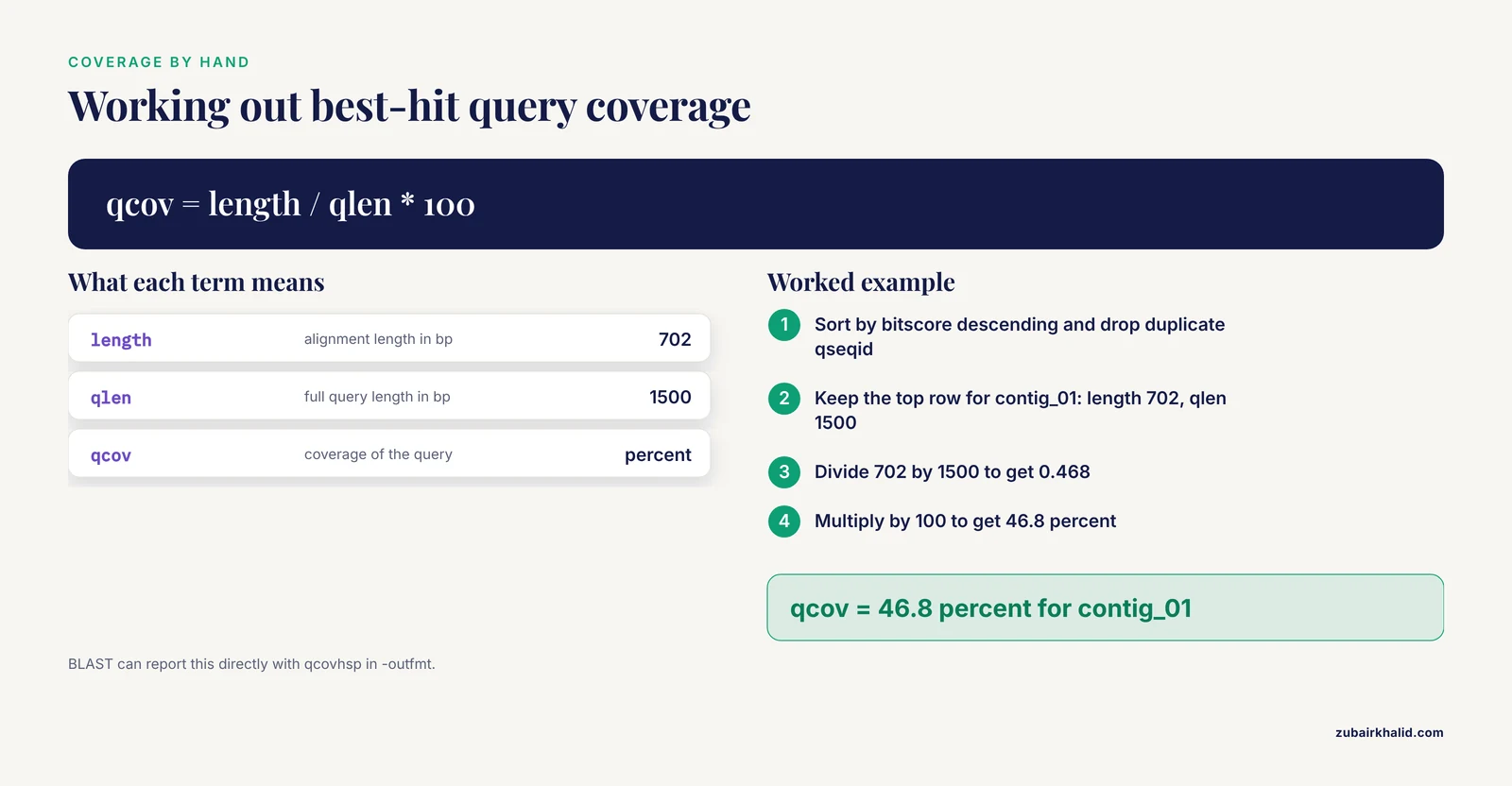
Coverage is the fraction of the query spanned by an alignment, and it separates a 70-base fragment match from a full-length hit with the same percent identity. For each query, take the single best HSP by bit score and compute coverage from the alignment length and the query length:
best = (hits.sort_values("bitscore", ascending=False)
            .drop_duplicates("qseqid", keep="first"))
best["qcov"] = best["length"] / best["qlen"] * 100

fig, ax = plt.subplots(figsize=(7, 4.5))
ax.hist(best["qcov"], bins=20, color="#64B5CD", edgecolor="white")
ax.set_xlabel("Best-hit query coverage (% of query length)")
ax.set_ylabel("Number of queries")
fig.tight_layout()
plt.show()
Expected shape: a peak near 100 percent for a clean search, with a left tail of partial hits that may be contig edges, fragmented genes, or sequence that does not belong.
BLAST can compute coverage for you. Add qcovhsp to -outfmt for per-HSP coverage, or qcovs for coverage aggregated over all HSPs of a query-subject pair. The manual calculation above matches qcovhsp for a single best HSP.
Step 9: Save the figures
Screenshots are not figures. Save every plot programmatically, at print resolution, in both raster and vector form:
fig.savefig("evalue_distribution.png", dpi=300, bbox_inches="tight")
fig.savefig("evalue_distribution.pdf", bbox_inches="tight")
PNG at 300 dots per inch suits slides and documents. PDF and SVG are vector formats that stay sharp at any size and are what most journals prefer. Call savefig before plt.show(), because show() clears the figure in some backends.
Practical tips for readable distribution plots
- Put units in axis labels, for example "Alignment length (bp)" rather than "Length".
- Start with 30 to 40 bins, then adjust. Too few bins hides subpopulations, too many bins turns noise into cliffs.
- Keep one consistent color scheme across all plots in a report so readers stop relearning the legend.
- Use alpha between 0.5 and 0.8 on dense scatters so overlapping points stay visible.
- Log-transform any variable that spans orders of magnitude, and say so in the axis label.
- Record the BLAST command, database name, and
blastnversion in the figure caption or a log file, because a distribution is meaningless without the search context. - If you prefer seaborn,
sns.histplotis a drop-in replacement forax.histwith nicer defaults.
Key Options and Formulas at a Glance
| Plot | Question it answers | Core code | Watch out for |
|---|---|---|---|
| log10(E-value) histogram | How strong are the hits overall? | np.log10(ev) then ax.hist | 0.0 E-values break log10, replace with NaN first |
| Bit score histogram | How does alignment quality spread? | ax.hist(hits["bitscore"], bins=40) | Safer than E-value for comparing across searches |
| Percent identity histogram | Are there close and distant populations? | ax.hist(hits["pident"], bins=40) | Identity says nothing about coverage |
| Hits per query | Which queries are promiscuous or silent? | hits.groupby("qseqid").size() | Zero-hit queries are absent from the file |
| Identity vs length scatter | Where is the population structure? | ax.scatter(length, pident, c=bitscore) | Overplotting above roughly 10,000 points, use hexbin |
| Best-hit coverage | Are hits full length? | length / qlen * 100 after best-hit selection | Per-HSP coverage differs from per-subject coverage (qcovs) |
A Short Biopython Route for XML Output
Many pipelines store BLAST results as XML (produced with -outfmt 5), and any Biopython tutorial you have followed probably ended by printing hits from that XML. The step from printed hits to plottable numbers is small. For a quick look, use the classic parser:
from Bio.Blast import NCBIXML

for result in NCBIXML.parse(open("hits.xml")):
    for alignment in result.alignments:
        for hsp in alignment.hsps:
            print(alignment.hit_id, hsp.expect, hsp.score)
For whole-file parsing into a DataFrame, SearchIO scales better and exposes consistent attribute names:
import pandas as pd
from Bio import SearchIO

rows = []
for qresult in SearchIO.parse("hits.xml", "blast-xml"):
    for hit in qresult:
        for hsp in hit:
            rows.append({
                "qseqid": qresult.id,
                "sseqid": hit.id,
                "evalue": hsp.evalue,
                "bitscore": hsp.bitscore,
                "pident": hsp.ident_num / hsp.aln_span * 100,
            })
hits = pd.DataFrame(rows)
From here, every plot in the walkthrough works unchanged. One caveat on speed: parsing is the slow step for large results, and the BLAST-QC authors benchmarked their purpose-built parser against parsers built on the commonly used BioPerl and Biopython modules and reported faster runtimes for their implementation [1]. If you routinely parse files with millions of lines, prefer tabular output read by pandas, which uses a C parsing engine, over XML read by Biopython, and use the chunksize argument of read_csv for files that exceed memory.
Fixing Common Errors
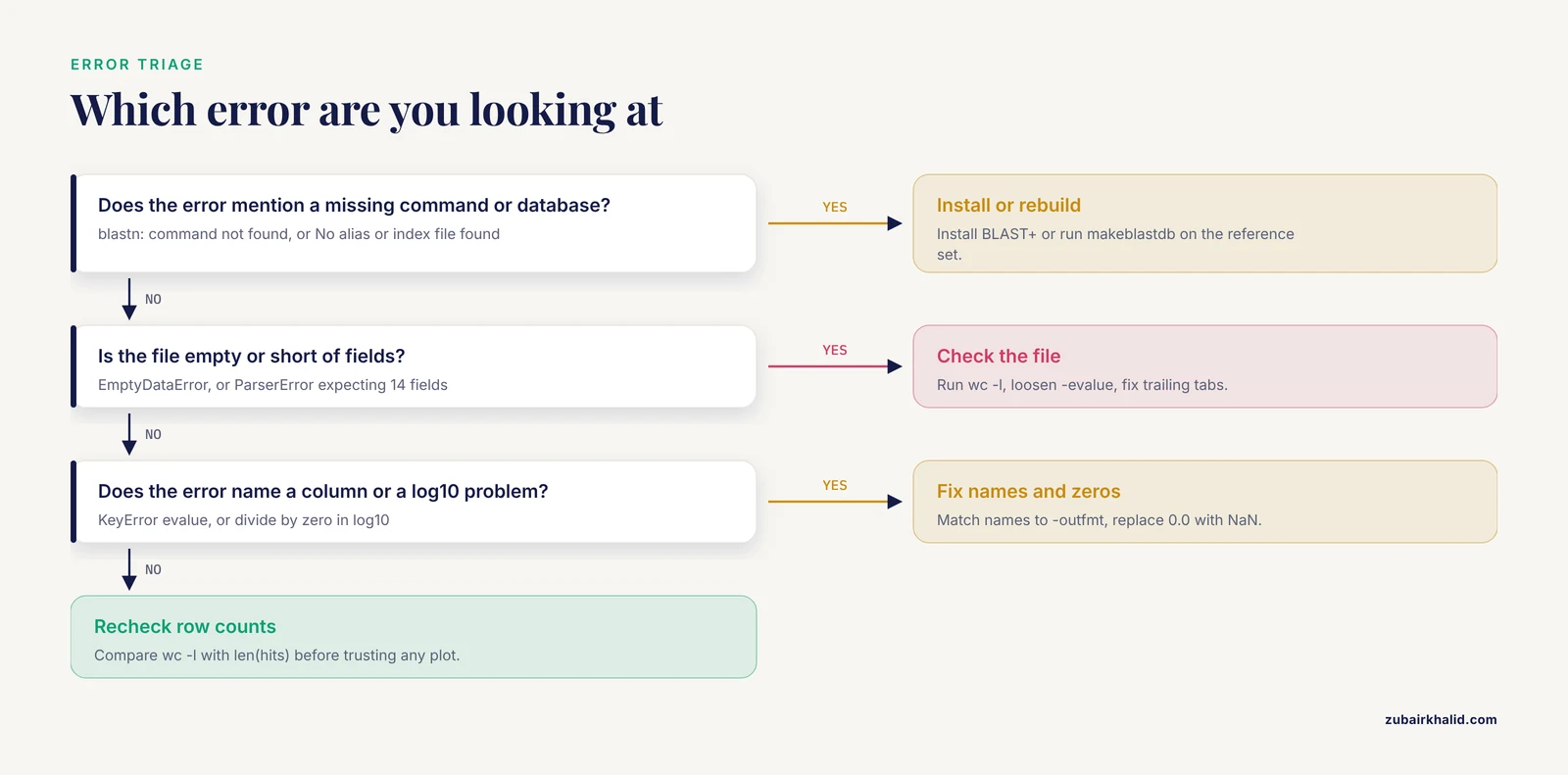
These are the failures you will actually hit, with the messages as they appear.
blastn: command not found. The BLAST+ executables are not installed or not on your PATH. Install them withconda install -c bioconda blastor from the NCBI BLAST+ download page at https://ftp.ncbi.nlm.nih.gov/blast/executables/blast+/LATEST/, then reopen the terminal.
BLAST Database error: No alias or index file found for nucleotide database [refseq_fungi] in search path [...]. The-dbvalue does not point at a formatted database. Either use the full path to the database prefix you created, or build one withmakeblastdb -in refs.fa -dbtype nucl -out /data/blast/refseq_fungi. Use-dbtype protfor protein databases searched withblastp.
FileNotFoundError: [Errno 2] No such file or directory: 'hits.tsv'. Python looked in its current working directory and found nothing. Check where you are withpwdin the terminal, or in Python:
import os
print(os.getcwd())
Then pass an absolute path such as /data/projects/blast/hits.tsv, or run BLAST and Python from the same directory.
pandas.errors.EmptyDataError: No columns to parse from file. The file exists but is empty, which almost always means BLAST found no hits at your-evaluethreshold. Check withwc -l hits.tsv, then rerun with a looser threshold such as-evalue 10to see whether anything appears at all.
pandas.errors.ParserError: Error tokenizing data. C error: Expected 14 fields in line 37, saw 15. One line has more tab-separated fields than your names list, usually from a trailing tab or a pasted header. Count fields per line withawk -F'\t' '{print NF}' hits.tsv | sort | uniq -c, fix the offending lines, and make sure the names list length equals the number of-outfmtfields.
KeyError: 'evalue'. The column name does not exist, typically because the names list does not match the file. Printhits.columnsand compare it with your-outfmtstring.
RuntimeWarning: divide by zero encountered in log10. You log-transformed a column containing0.0E-values. Apply the replace shown in Step 4 before the transform.
TypeError: ufunc 'log10' not supported for the input types. The column contains strings rather than numbers, which happens when the file was read with the wrong separator and everything landed in one column. Re-read withsep="\t"and verify withhits.dtypes.
- BLAST refuses the command with
BLAST query/options error: -outfmt: Unknown field: "qcov". You asked for a field name that does not exist. The valid coverage fields areqcovhspandqcovs, and the error output lists the accepted names, so copy from there.
How to Check That Your Plots Are Right
A plot can be beautiful and wrong. Four checks catch most problems.
First, reconcile row counts. wc -l hits.tsv in the terminal must equal len(hits) in pandas. If they differ, you parsed a partial file.
Second, enforce physical constraints:
assert (hits["pident"] <= 100).all()
assert (hits["evalue"] >= 0).all()
assert (hits["length"] <= hits[["qlen", "slen"]].min(axis=1)).all()
An alignment cannot be longer than the shorter of the two sequences, and identity cannot exceed 100. A failed assert points at a parsing error, not at BLAST.
Third, confirm that E-value and bit score ordering agree, because within a single search they carry the same information:
print(hits["evalue"].corr(hits["bitscore"], method="spearman"))A Spearman correlation close to -1 is expected, since higher bit scores go with smaller E-values. A weak correlation means something is wrong with the parse.
Fourth, spot-check one row against the default BLAST output. Run blastn on a single query without -outfmt, find the top hit, and confirm that the E-value and identity match the corresponding row in your DataFrame. This closes the loop between the search and the parser.
Record provenance alongside the figures: the output of blastn -version, the database name and build date, and the full command line. A distribution without that context cannot be interpreted or repeated.
Common Mistakes and Limitations
- Treating
-max_target_seqsas "give me the best N hits". The parameter caps reporting but interacts with the heuristic search, and its behavior has been questioned in the BLAST literature [1]. Your distributions describe the hits that were reported, which is not always the same as the best hits that exist. State the value in your methods.
- Plotting raw E-values on a linear axis. Everything from 1e-180 to 1e-10 collapses onto the zero line and the plot shows one bar. Always log-transform.
- Forgetting that BLAST prints
0.0for very small E-values. log10 of those values produces negative infinity and a phantom bar at the left edge. Replace zeros before transforming.
- Counting HSPs as independent hits. A query that matches one subject in three regions contributes three rows. If you want per-hit statistics, aggregate with
groupbyfirst, as in Step 8. Multi-region matches are a normal BLAST outcome, not an error [2].
- Ignoring queries with zero hits. They are absent from the output file, so every per-query plot silently excludes them. Compare against the query FASTA as in Step 6.
- Reading percent identity as coverage. A 99 percent identity match over 50 bases is usually less meaningful than an 85 percent match over 2,000 bases. Plot both metrics.
- Comparing E-values across searches against different databases. The E-value is scaled by the size of the database searched, so 1e-20 against a small reference set is not the same evidence as 1e-20 against nt. Use bit scores for cross-search comparisons.
- Overplotting large scatters. With hundreds of thousands of HSPs, a plain scatter draws a solid rectangle. Use hexbin or a two-dimensional histogram with a log color scale.
- Assuming the plots validate the biology. They validate the search and the parse. A clean distribution does not make a hit biologically meaningful, and orthology decisions need reciprocal analysis plus coverage and identity thresholds rather than an E-value alone.
- Parsing huge files line by line in pure Python. It works for megabytes and crawls for gigabytes. Use pandas with its C parsing engine and the
chunksizeargument, or a dedicated parser, when files grow.
Next Steps
Once the distributions look sane, the natural sequence is to filter the DataFrame with thresholds you can defend from the plots (for example bitscore above 50 and coverage above 70 percent), aggregate to one best hit per query, then hand the filtered table to annotation or clustering. If the goal is orthology between two sequence sets, the standard BLAST-based approach is to search all sequences against all and retrieve reciprocal best hits, the exact use case the PARIGA server was built to manage with interactive filtering [2]. Keep the notebook and the raw hits.tsv, rerun the plots after any parameter change, and let the shapes rather than single numbers drive the thresholds.
Frequently Asked Questions
Do I need Biopython to visualize BLAST hits in Python?
No. Pandas and matplotlib handle tabular BLAST output on their own, and that is the fastest route. Biopython earns its place when your results are in XML, when you need to count zero-hit queries from the FASTA file, or when you want programmatic access to the alignments themselves.
Which BLAST output format should I use for plotting?
Use -outfmt 6 with an explicit field list that includes qlen and slen. Format 6 is tab-separated with no header, so pandas reads it in one line. Format 7 adds comment lines you must strip, and the default pairwise format is not practical to parse. If you run BLAST in a browser, download the tabular hit table and start at Step 2.
Why does my E-value histogram look empty or pile up at zero?
Because E-values span many orders of magnitude and a linear axis crushes them into one bin. Take log10 of the E-values first, and replace the 0.0 values that BLAST prints for extremely small E-values with NaN before the transform.
How do I plot only the best hit for each query?
Sort by bitscore in descending order and drop duplicate query identifiers with hits.sort_values("bitscore", ascending=False).drop_duplicates("qseqid"). That keeps one row per query, the highest-scoring HSP, which is what most best-hit plots need.
Can I run this workflow in Google Colab?
Yes. Upload hits.tsv or mount Google Drive, then run the same pandas and matplotlib code in a notebook. Most people run the BLAST search itself locally or on a server and do the plotting in Colab.
How many bins should I use for a BLAST histogram?
Start with 30 to 40 bins and adjust by eye. Too few bins merges distinct populations and too many bins turns random noise into apparent structure. For a data-driven choice, pass bins="auto" to apply standard rules such as Freedman-Diaconis.
How do I draw hits along the subject sequence?
Use the sstart and send columns to draw one rectangle or line per HSP along an x-axis that represents the subject, stacking queries on the y-axis with matplotlib patches. This produces an alignment map that makes multi-region matches obvious.
Are distribution plots enough to pick orthologs?
No. The plots screen the search and expose structure, but orthology calls need reciprocal best hit analysis plus coverage and identity thresholds applied to the filtered hits. Use the plots to choose the thresholds, not to make the call itself.