How to Validate Bioinformatics Pipelines After Cloud Migration
By Dr. Zubair Khalid, DVM, MS, PhD ·

By the end of this guide you will be able to prove, with files and numbers you can hand to a reviewer, that a bioinformatics pipeline running in the cloud produces the same biological results it produced on your old on-premises servers. You will build a golden dataset, freeze software versions, run the migrated pipeline on cloud infrastructure, compare outputs against reference results, and write a validation report that a collaborator, a QA officer, or an auditor can actually follow.
This guide assumes a standard next-generation sequencing workflow (alignment plus variant calling) as the worked example, but the same method applies to RNA-seq quantification, metagenomic classification, assembly, or any other reproducible analysis. The stakes are real. Human genomics work presented at community meetings such as the Human Genome Meeting 2016 spanned phenome-wide association studies across tens of thousands of participants, methylation analyses in birth cohorts, and single-cell allele-specific expression in aneuploidy research [1]. Every one of those analysis types depends on pipelines that return the same answer regardless of where they run.
What you need on hand before you start
Gather these before touching the cloud console:
- A pipeline that runs end to end on your current system, packaged with Nextflow, Snakemake, WDL (Cromwell), or plain shell scripts.
- Version pins for every tool and every container image, captured as digests rather than tags.
- Two to five test samples that cover your real data diversity (different read lengths, coverage levels, library types, or organism references if you run several).
- Reference outputs produced by the pipeline on your original system, stored somewhere safe and unchangeable.
- A cloud account with permissions to create storage, compute, and batch resources. The worked commands assume AWS (S3 for storage, EC2 or AWS Batch for compute), since aws genomics is the most common migration target, but the logic transfers directly to Azure Batch, Google Cloud Life Sciences, or an HPC cloud appliance.
- The AWS CLI, Nextflow or your chosen workflow engine, samtools, bcftools, and ideally RTG Tools for variant comparison, installed on a machine you control.
Nothing in this guide requires proprietary software. Everything shown runs with open source tools and standard cloud services.
Why validation changes when a pipeline moves to the cloud
On your old server, the pipeline, the operating system, the reference files, and the hardware all stayed fixed. After a migration, up to five things change at once:
- Compute hardware. A c5 instance has different CPU instructions and memory bandwidth than your departmental server. Most bioinformatics tools give bit-identical results across reasonable x86 hardware, but multithreaded tools with non-deterministic reduction order can produce small floating point differences.
- Storage layout. Reading FASTQ files from S3 object storage instead of a local filesystem changes I/O behavior. This affects speed, not correctness, unless a transfer silently corrupts a file.
- Container images. A tag like
biocontainers/samtools:v1.9can be rebuilt upstream. If your cloud run pulls a rebuilt image, you are validating a different program. - Scheduling behavior. Cloud batch systems retry failed tasks, sometimes on Spot instances that get reclaimed mid-run. A task that resumes or retries must produce the same output as a clean run.
- Reference data placement. A reference genome copied to S3 can be corrupted, truncated, or replaced by the wrong assembly build without anyone noticing until results drift.
Validation after migration therefore answers one question with evidence: do the outputs match, byte for byte where possible, and biologically everywhere else?
Step-by-step validation walkthrough
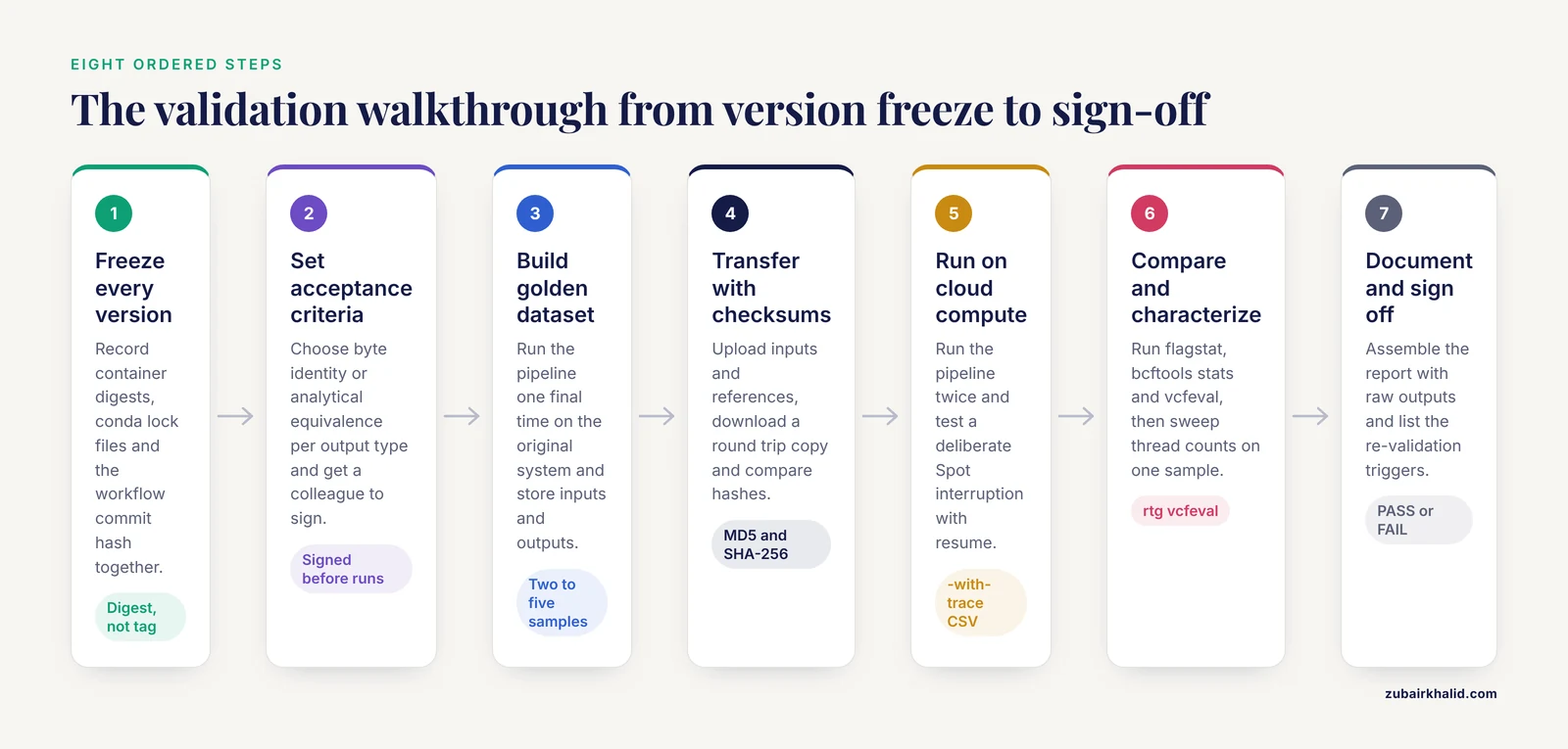
The steps below are ordered. Skipping a step almost always costs more time later than it saves.
Step 1. Freeze and record every version
Write down exactly what runs. For container images, record the digest, not the tag:
docker inspect biocontainers/bwa:v0.7.17_cv1 \
  --format '{{index .RepoDigests 0}}'
Expected output (your digest will differ):
biocontainers/bwa:v0.7.17_cv1@sha256:1ac2d8a2ff00ef5ed4a2e5b2f5b2a9c9e0d8a5f0b3d1a7e4c2f8b6d9e1a3c5f7For conda-based tools, export a lock file:
conda list --explicit > env-lock-2026-11-11.txtFor the workflow itself, record the commit hash:
git -C my-pipeline rev-parse HEADExpected output:
3f9c1a2b7d4e5f60718293a4b5c6d7e8f9012a3bSave these three records together. If a reviewer asks in eight months which bwa ran the validation, the digest answers in seconds. A tag answers nothing, because tags move.
Step 2. Define acceptance criteria before running anything
There are two levels of agreement, and you should choose them per output type before you run anything.
- Byte identity. The output file has the same SHA-256 hash as the reference. Appropriate for deterministic text outputs such as most VCF files (after header normalization) and summary tables.
- Analytical equivalence. The outputs differ in bytes but not in biological content. Appropriate for BAM files (headers embed command lines and local paths) and for any output influenced by thread count.
Write the criteria as a short table and get a colleague to sign it. An acceptance criterion written after seeing the results is not validation, it is rationalization.
Step 3. Build the golden dataset and reference outputs
Pick your test samples, run the full pipeline on the original system one final time, and store everything:
mkdir -p golden/input golden/output
cp sample_A_R1.fastq.gz sample_A_R2.fastq.gz golden/input/
cd golden/output
md5sum * > ../golden.md5
Expected content of golden.md5:
d41d8cd98f00b204e9800998ecf8427e  sample_A.sorted.bam
67e4b7c8e9f0a1b2c3d4e5f60718293a  sample_A.variants.vcf.gz
Keep a copy of the reference outputs somewhere the migration cannot touch, such as a second storage bucket or a lab archive server, with write access removed. The golden outputs are the arbiter of truth for the entire exercise. If you lose them, you restart from your original system.
Step 4. Transfer data with integrity checks
Upload the golden inputs to cloud storage and verify the transfer. For files under a few gigabytes, checksum comparison is straightforward:
md5sum golden/input/sample_A_R1.fastq.gz
aws s3 cp golden/input/sample_A_R1.fastq.gz \
    s3://my-lab-bucket/validation/input/
aws s3 cp s3://my-lab-bucket/validation/input/sample_A_R1.fastq.gz /tmp/roundtrip/
md5sum /tmp/roundtrip/sample_A_R1.fastq.gz
Both hashes must match. For large files, download a round trip copy and hash it rather than trusting the upload. S3 multipart uploads make the object ETag differ from the file MD5, which confuses many people, so compare hashes on a downloaded copy instead of reading the ETag from the console.
Do the same for reference genomes and known indices:
sha256sum homo_sapiens_GRCh38.fa* > reference.sha256
aws s3 cp reference.sha256 s3://my-lab-bucket/references/GRCh38/
A wrong or truncated reference file is the single most damaging silent failure in cloud bioinformatics, and it is completely preventable with this five-minute check.
Step 5. Run the pipeline on cloud compute
For a Nextflow pipeline with an aws batch profile:
nextflow run main.nf \
  -profile awsbatch \
  --input 's3://my-lab-bucket/validation/input/*_{R1,R2}.fastq.gz' \
  --outdir s3://my-lab-bucket/validation/output \
  -with-report validation_report.html \
  -with-trace validation_trace.csv
Parameters that matter here:
-profile awsbatchselects the cloud executor and container definitions defined in your config. Runnextflow config -profile awsbatchfirst and read the output. Confirm queue names, regions, and work directory paths.-outdiron S3 keeps results durable. Local scratch on the compute node disappears with the instance.-with-traceproduces a per-task CSV with real CPU hours, memory peaks, and exit codes. This file becomes part of your validation evidence.
Expected trace rows look like:
task_id    status    exit    process        cpus    peak_rss_megs
2ab1x9     OK        0       ALIGN_BWA      8       14210
2ab1yb     OK        0       SORT_INDEX     2       3120
2ab1z4     OK        0       CALL_VARIANTS  4       8730
Run the pipeline twice on the same inputs during validation. The first run proves it works. The second run proves outputs are stable when nothing changed, which is the property your reviewers actually care about. This is also the right time to test a Spot interruption deliberately, either by requesting a two-minute interruption window in a test or by cancelling and resuming with nextflow run -resume, then confirming the final outputs still match the reference.
Step 6. Compare outputs against the reference
Run the full comparison battery. The table below summarizes the core checks.
| Check | Tool | Command | Pass criterion |
|---|---|---|---|
| Fastq integrity | md5sum | md5sum -c golden.md5 | All files report OK |
| Alignment counts | samtools | samtools flagstat sample_A.bam | Identical totals for mapped, paired, duplicate lines |
| Alignment checksum | samtools + sha256sum | Hash of samtools view output with header stripped | Identical to reference hash |
| Variant counts | bcftools | bcftools stats ref.vcf.gz cloud.vcf.gz | Identical record counts per sample |
| Variant concordance | RTG Tools | rtg vcfeval -b ref.vcf.gz -c cloud.vcf.gz | Zero false positives and false negatives, or within your pre-set tolerance |
| Summary tables | diff | diff ref_summary.csv cloud_summary.csv | No differences |
A header-normalized BAM data hash is the strongest alignment check:
samtools view -h sample_A.cloud.bam | \
  grep -v '^@PG' | \
  sha256sum
Run the identical command on the reference BAM. Stripping the @PG lines removes command-line records that legitimately change between systems (they embed local paths). If the hashes now match, your alignments are byte-identical where it matters.
For variants:
rtg vcfeval -b golden/sample_A.ref.vcf.gz \
            -c cloud/sample_A.cloud.vcf.gz \
            -o vcfeval_out --squash-ploidy
Expected summary (illustrative values, your numbers come from your data):
Eval/baseline variant comparison summary
True positive baselines:   4,912,207
True positive calls:       4,912,210
False positives:               3
False negatives:               0
If false positives and false negatives are all zero, stop. Byte-equivalent variant calls are a perfect result. If there is a small nonzero count, do not wave it through. Diff the discordant records with bcftools view -H on the RTG output files, look at the genotypes and positions, and decide whether the differences come from a real algorithmic change (fail) or from a documented, bounded numerical difference you characterized in Step 7 (conditional pass, with the reasoning written down).
Step 7. Characterize runtime-driven differences deliberately
Some pipelines will never give byte-identical output across systems, and you need to know that now rather than during a production incident. The usual suspects:
- Tools with multithreaded floating point reduction, where the order of additions depends on thread count. Changing the requested CPU count can change low-order digits in quality scores or abundance estimates.
- Tools that embed timestamps, hostnames, or temporary paths in output headers.
- Compressed outputs where the compression library version differs, producing different bytes that decompress to identical content.
To characterize this, rerun the cloud pipeline with different thread counts on one sample and hash the outputs:
nextflow run main.nf -profile awsbatch --max_cpus 4  --outdir s3://my-lab-bucket/validation/c4
nextflow run main.nf -profile awsbatch --max_cpus 16 --outdir s3://my-lab-bucket/validation/c16
If the variant content is identical across thread counts but compression bytes differ, your acceptance criterion for those files should be analytical equivalence via bcftools stats and vcfeval, not raw MD5. If variant content itself shifts with thread count, that tool needs a fixed thread count written into the pipeline config, and the validation rerun confirms the fix.
Step 8. Document, sign off, and define re-validation triggers
A validation that lives only in someone's terminal history does not exist. Produce one document containing:
- The version freeze from Step 1 (digests, commit hashes, conda lock files).
- The acceptance criteria table from Step 2, signed before runs.
- The comparison results from Step 6, including raw tool outputs as attachments.
- The trace CSV showing resource usage and exit codes.
- The thread count characterization from Step 7, if any output was granted analytical equivalence.
- A list of named re-validation triggers: any container image change, workflow code change, reference file replacement, executor change, or region change that affects compute generation.
Common errors, their exact messages, and fixes
These are the failures you will actually hit, with the strings that appear in your logs:
Unable to locate credentialsfrom the AWS CLI or boto3. The task ran without an attached IAM role. Fix by attaching a role to the Batch compute environment or EC2 instance profile, not by baking keys into images.Permission denied (publickey)when a process tries to reach another node. The batch environment security group or SSH key setup is wrong. For most workflows the fix is to remove SSH dependencies entirely and use the workflow engine's native communication.Command exited with status 137in a Nextflow or Snakemake task log. Exit code 137 means the process was killed, almost always the Linux out-of-memory killer after the container exceeded its memory limit. Raise the task memory request in the process config and rerun. Do not treat a successful rerun as validation evidence for the failing configuration.No space left on devicein a task's stderr. The scratch volume or work directory filled up. Check whether your config requests an ephemeral volume large enough for intermediate files, or direct intermediate files to instance store volumes sized for the workload.EntityTooLargefrom a direct S3 PUT. A single non-multipart upload exceeded the 5 GB limit. Useaws s3 cp(which handles multipart automatically) instead ofaws s3api put-objectfor large files.manifest unknownfrom a container pull. The tag was deleted or rebuilt upstream. This is exactly why Step 1 records digests. Pin the digest and the pull succeeds deterministically.
Common Mistakes and Limitations
These are the errors that show up repeatedly when teams validate cloud-migrated bioinformatics pipelines:
- Validating only the happy path. A single clean run proves the pipeline works once. Run it twice, run it with a deliberate Spot interruption and resume, and run it on your largest and smallest test samples.
- Comparing MD5 hashes of BAM files and declaring failure. BAM headers embed command lines with absolute paths, which legitimately change between systems. Hash the header-stripped alignment data, or you will chase a non-problem for a day.
- Pinning tags instead of digests. A floating container tag can be silently rebuilt between your on-premises run and your cloud run. Your validation then compares two different programs and concludes the cloud broke something, or worse, that it did not.
- Copying reference data without checksums. A corrupted or wrong-build reference in S3 produces plausible-looking results with systematic errors. Always upload a checksum manifest and verify before the first production run.
- Treating a longer runtime as a validation failure. Cloud tasks run slower or faster than local ones for many reasons including I/O and instance generation. Validation compares correctness, not wall clock. Use the trace file to record runtimes for cost planning, separately from the correctness verdict.
- Writing acceptance criteria after seeing results. Decide before running what counts as a pass. Retroactive thresholds are the most common way validation becomes theater.
- Forgetting the downsampling behavior of test data. If your test samples are tiny, rare failure modes tied to large files (multipart uploads, memory paging on deep coverage) go untested. Include at least one production-scale sample if budget allows.
- Skipping documentation because everything matched. A perfect byte-identical result with no recorded versions and no signed criteria is not reproducible evidence. Future auditors cannot reconstruct what you proved.
One structural limitation applies to this entire guide: validation establishes that a pipeline reproduces defined reference results on defined test data. It does not establish that the pipeline is biologically correct for new data types you have never run. Validation is repeatable after every material change, and the trigger list in Step 8 is what keeps it honest.
Reading Your Comparison Output Field by Field
The step-by-step walkthrough tells you which tools to run. This section tells you how to read what they print, because the difference between a pass and a false alarm usually lives in one line of tool output.
Interpreting samtools flagstat
A typical pair of flagstat outputs looks like this:
On-premises reference            Cloud run
4912234 + 0 in total              4912234 + 0 in total
2456117 + 0 paired in sequencing  2456117 + 0 paired in sequencing
1229290 + 0 read1                 1229290 + 0 read1
1226827 + 0 read2                 1226827 + 0 read2
4852101 + 0 properly paired       4852101 + 0 properly paired
4898011 + 0 with itself and mate mapped  4898011 + 0 with itself and mate mapped
3999 + 0 singletons               3999 + 0 singletons
0 + 0 with mate mapped to a different chr  0 + 0 with mate mapped to a different chr
246118 + 0 duplicates             246118 + 0 duplicates
Read the lines in a fixed order and compare each one deliberately. Total reads first: a difference here almost always means the input FASTQ was not identical, which points back to a transfer problem rather than a compute problem. Properly paired and singletons next: a shift here with identical totals suggests the alignment itself changed, which points to a reference genome difference, an index difference, or a parameter difference. Duplicate counts last: duplicate marking can be sensitive to the order in which reads reach the marker in some implementations, so a small duplicate count difference is a known analytical equivalence candidate rather than an automatic failure, provided your acceptance criteria said so before the run.
A practical habit is to paste both outputs into the validation report side by side. Reviewers trust what they can see, and the side-by-side layout makes a single differing line jump out.
Interpreting bcftools stats
Run the two callsets through the same command:
bcftools stats sample_A.ref.vcf.gz sample_A.cloud.vcf.gz > compare.statsThen walk the report top to bottom. The record count lines near the top tell you whether the two files contain the same number of variants per sample. If those match, continue to the per-quality metrics and the transition to transversion summary further down. If record counts differ, everything below is less informative until you know which records are missing, which is exactly what rtg vcfeval tells you. In practice, read the summary lines first for a quick verdict, then use the detailed sections to characterize any mismatch before you open a single VCF record by hand.
Interpreting rtg vcfeval
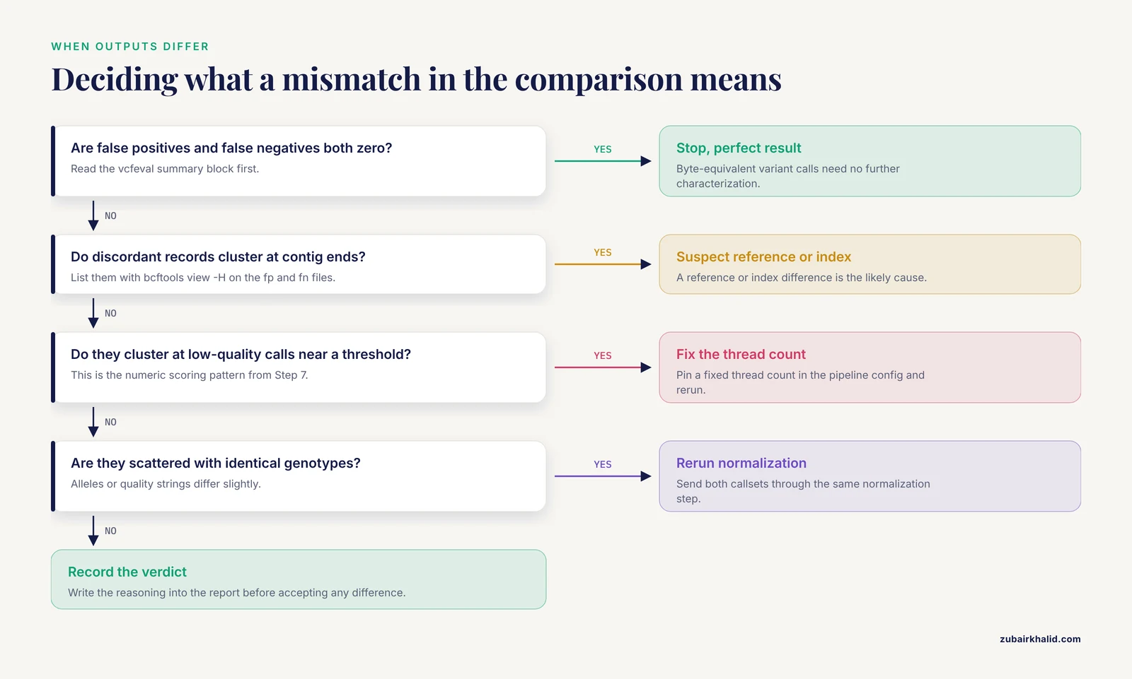
The summary block groups records into true positives, false positives, false negatives, and their variants. The two numbers that decide your verdict are false positives (calls present in the cloud output but not the reference) and false negatives (reference calls the cloud output missed). A nonzero count in either column means at least one record differs. The next move is never to average it away. List the discordant records, which vcfeval writes to files in its output directory, and inspect them:
bcftools view -H vcfeval_out/tp-baseline.vcf.gz | head
bcftools view -H vcfeval_out/fp.vcf.gz
bcftools view -H vcfeval_out/fn.vcf.gz
Three mismatch patterns recur, and each has a different diagnosis. If the discordant records cluster at the start or end of contigs, suspect a reference or index difference. If they cluster at low-quality calls near some threshold, suspect a numeric difference in scoring, which is the thread count or library version pattern described in Step 7 of the main walkthrough. If they are scattered randomly with identical genotypes and slightly different alleles or quality strings, suspect a normalization difference, and rerun both callsets through the same normalization step before comparing again.
A quick word on what "identical" means for summary tables
The diff check on summary tables is binary, but resist the temptation to eyeball a diff and declare the changed lines unimportant. Every changed line must be explained in writing. If the explanation is a timestamp column, that is an analytical equivalence with a documented reason. If the explanation is "the numbers are close," that is a failure you have not characterized yet.
Bisecting a Mismatch: A Stage-by-Stage Debugging Protocol
When the final outputs do not match and the cause is not obvious, the fastest path to an answer is bisection. The principle: run each pipeline stage individually against the golden inputs on both systems, hash the intermediate output of each stage, and find the first stage where the hashes diverge. Everything upstream of the divergence is innocent; the fault lives in the first divergent stage or in its inputs.
A concrete protocol:
- List the stages of your pipeline in order, for example: quality control, trimming, alignment, sorting and indexing, duplicate marking, variant calling.
- On the original system, run each stage separately and save every intermediate file, with a checksum manifest for the intermediates.
- On the cloud system, run the same stages separately with the same pinned containers and the same parameters, saving intermediates the same way.
- Walk the manifest from the top and stop at the first checksum mismatch.
Suppose trimming outputs match, alignment outputs match, and duplicate marking outputs diverge. Your search space just collapsed from the whole pipeline to one process. Now interrogate that process:
- Confirm the container digest is the same on both systems. A silently rebuilt image is the most common cause of a single-stage divergence.
- Confirm the command line is identical, character for character. Sorting or duplicate marking tools sometimes receive a thread count or memory setting from the workflow config that differs between your old scheduler and the cloud batch queue.
- Confirm the input to the stage on the cloud system decompresses to the same bytes as the input on the original system. A round-trip download and hash removes all doubt.
- Rerun the stage alone twice on the cloud system. If two cloud runs disagree with each other, the problem is non-determinism inside the tool, not the migration.
If every stage matches individually but the assembled pipeline still produces different finals, look at the workflow glue: file naming, glob patterns that pick up the wrong intermediate, or a task that ran against a stale work directory. This failure mode is rarer than a tool-level difference but it does happen, and the trace CSV from your workflow engine is the evidence that shows which file each task actually consumed.
One caution: do not "fix" a mismatch by editing the pipeline mid-validation. Any change to code, parameters, or containers invalidates the runs you already did, and the honest response is to restart the affected comparison from the top with the change recorded in the version freeze. This feels slow and it is, but a validation report that mixes pre-change and post-change results is worse than no report, because it looks authoritative while proving nothing.
Choosing a Pinning Strategy: Tags, Digests, Lock Files, and Frozen Images
Step 1 of the walkthrough tells you to record digests. This section compares the pinning strategies available to you, because teams routinely pick one that does not match how their pipeline actually runs, and the mismatch shows up as a failed validation months later.
| Strategy | What it pins | Strength | Weakness | Best suited to |
|---|---|---|---|---|
| - | - | - | - | - |
| Floating tag | Whatever the registry serves | Zero effort | Silently rebuilt images; deleted tags | Nothing in validation |
| Digest pin | Exact image bytes | Byte-level reproducibility | Digests differ across registries even for identical content; mirroring needed for durability | Validation runs and production |
| Conda lock file | Exact package builds | Works without containers | Solver output must actually be frozen and reused, not regenerated | Teams standardized on conda or mamba |
| Apptainer or Singularity SIF | A single immutable image file | File lives in your storage, immune to registry changes | Large files; you must manage storage lifecycle | HPC-adjacent cloud setups |
| Custom machine image (AMI and equivalents) | OS, drivers, and tools together | Removes OS-level drift | Heavier to rebuild and audit per change | Validation of instance-sensitive tools |
| Workflow engine module pins (for example, nf-core module versions) | Tool plus tested invocation | Community-tested combinations | Still depends on the underlying container pin | Nextflow and Snakemake pipelines using community modules |
Three practical notes on the table. First, the digest weakness matters more than most people expect: the same image content can have different digests in different registries, so if your validation report records a digest from one registry and your cloud config pulls from another, you need a documented mapping between them, or a mirrored copy in a registry you control. Second, a lock file only helps if your pipeline actually installs from the lock file at run time. Regenerating the environment on the fly from a loose specification reintroduces the drift you were pinning against. Third, a custom machine image is the heavyweight option, and it earns its weight in one specific situation: when you have established in Step 7 characterization that a tool's output shifts with CPU generation and you want the validation environment frozen at the hardware level as well as the software level.
Whichever strategy you choose, the validation test is the same: pull or build the environment fresh on the cloud system, record what you got, and confirm the record matches the version freeze from Step 1. If your pipeline logs the image digest or environment hash per task, extract those lines from the logs and attach them to the report. If it does not, add that logging before validation, because it turns every future audit question into a grep.
Where Non-Determinism Hides in Bioinformatics Tools
Step 7 of the walkthrough names the usual suspects. This section goes deeper, because knowing the mechanisms lets you predict which outputs need characterization before you ever run the comparison, and lets you write acceptance criteria that anticipate reality rather than discover it.
Thread-order floating point reduction. Tools that accumulate floating point values across threads, such as abundance estimators in quantification workflows or some quality recalibration steps, can produce low-order digit differences when the number of threads changes, because the additions happen in a different order and floating point addition is not associative. The signal to look for: hashes differ, but bcftools stats or a numeric comparison shows differences only in the last few significant digits of scores or estimates. The fix is a fixed thread count for that tool in the pipeline config, followed by a rerun of the comparison.
Hash iteration and set ordering. Some tools iterate over hash tables when writing output, and table iteration order can depend on insertion order or on memory addresses. The classic symptom is output lines that are correct individually but in a different order between runs. If a sort of both files makes them identical, the tool is non-deterministic only in ordering, and your acceptance criterion can be "identical after canonical sorting" with the sorting step recorded.
Compression library differences. BGZF and gzip outputs depend on the compression library version, the compression level, and sometimes the block size in memory at write time. Two files can decompress to identical content while hashing differently. This is why the acceptance framework in the main guide separates byte identity from analytical equivalence: for compressed outputs where the decompressed content is what matters, hash the decompressed content or compare content directly, and record the compression bytes as non-comparable.
Embedded provenance in headers. BAM @PG lines, VCF header lines, and the headers of many summary formats record command lines, working directories, hostnames, and timestamps. The main guide shows the @PG stripping pattern for BAMs. The general lesson is bigger: for every output type in your pipeline, know exactly which header fields are provenance and which are data, and write your comparison to ignore provenance and hash data. Do this once per output type and you will never chase a false alarm from a path string again.
Locale and collation in sorting. Sorting behavior can vary with locale settings if a tool shells out to system utilities. Pinning the container usually removes this risk, but if any task runs on the host rather than in a container, set the locale explicitly in the pipeline config and record it in the version freeze.
A compact characterization exercise covers most pipelines. Take one sample, one tool at a time, and run each of these comparisons on your cloud setup: same tool twice, tool with two thread counts, tool with two compression levels if applicable. The results give you a per-output-type verdict that feeds directly into the Step 2 acceptance table. Teams that skip this exercise usually discover their non-determinism during a production incident instead, at far higher cost.
Golden Dataset Design Beyond the Obvious
The main guide says to pick two to five samples covering your real data diversity. That sentence hides most of the design work, so here is how to actually choose and document the set.
Cover the axes that change your results. For a variant calling pipeline on human data, the axes that historically change results include read length, coverage, insert size distribution, library type, ancestry-informed reference allele frequencies in the panel used by joint calling steps, and regions that stress the aligner. You do not need a sample for every combination. You need the set, taken together, to touch every axis at least once. If your production work spans whole genome, exome, and targeted panels, at minimum include one genome-scale sample and one targeted sample, because they stress different parts of the pipeline.
Include the sample that broke something before. Teams accumulate war stories: the sample with an unusual contig naming mismatch, the sample that blew up the memory request, the sample with contamination that triggered an unexpected path through the QC logic. If such a sample exists in your history, it belongs in the golden set. A golden dataset that only contains easy samples validates the easy path.
Capture metadata with the data. For each golden sample, record in a small manifest: the source, the read length and layout, the coverage or approximate depth, why the sample was included, and the date the reference outputs were generated. Six months later, when someone asks why sample C is in the set, the manifest answers in seconds and the validation stays defensible.
Protect against sample swaps. Label every golden file consistently and store the manifest hashes alongside. Sample swaps during migration are rare but catastrophic, and a manifest with per-file hashes and sample identifiers makes any swap immediately visible at the Step 4 integrity check rather than three stages deep into debugging.
Size the set against your tolerance for validation cost. More samples means more compute and more comparison work, and also more coverage of failure modes. A reasonable compromise many teams land on: two or three small, fast samples for rapid iteration during debugging, plus one production-scale sample that runs only after the small ones pass. This keeps the expensive run for the moment when the cheap runs are clean.
Remember what the golden set is for. It is the arbiter of truth for the migration. The same reasoning about analysis diversity applies to your real production workload: population-scale association work, methylation analyses in cohorts, and single-cell analyses each stress pipelines differently, and community-scale genomics projects such as those presented at the Human Genome Meeting 2016 spanned exactly this range from phenome-wide association across tens of thousands of participants to methylation in birth cohorts and single-cell allele-specific expression [1]. Your golden set cannot cover all of that, so define its scope explicitly in the acceptance criteria: the validation proves equivalence for the data types the golden set represents, and the re-validation trigger list covers extensions beyond it.
Safe Reference Data Handling in Object Storage
The main guide covers checksum manifests at upload time. Three additions make reference data handling durable rather than a one-time check.
Turn on versioning for reference buckets. Object versioning means an accidental overwrite does not destroy the correct file; it creates a new version you can detect and roll back. Combined with the checksum manifest, a verification job that rehashes the current object versions against the manifest catches both corruption and replacement. The manifest itself belongs in the same bucket with versioning on, and ideally with access controls that make the reference prefix read-only for the compute roles that run pipelines.
Separate reference storage from run storage. A layout where references live under one prefix with restricted write access, and pipeline work directories live elsewhere, prevents the most damaging accident: a pipeline task or a human writing over a reference file during a run. If your workflow config points at a reference path, that path should resolve to storage that only a deliberate administrative action can modify, and that action should be a re-validation trigger by definition.
Re-verify on a schedule, not just once. Silent corruption in object storage is rare, but the realistic risk is human: a colleague re-uploads a reference with a slightly different preparation, or a script writes to the wrong prefix. A scheduled job that downloads each reference, hashes it, and compares against the manifest turns a silent drift into a detected event. Attach the job output to your validation records so the evidence chain stays continuous between formal validations.
The five-minute checksum check in the main walkthrough prevents the worst single failure. Versioning, separation, and scheduled re-verification extend that check into a system that keeps working after everyone has moved on to the next migration task.
Testing Retry Behavior and Spot Interruption in Detail
The main guide tells you to run the pipeline twice and to test a deliberate interruption. Here is the detailed procedure, because retry behavior is where cloud pipelines differ most from the single long-running jobs of an on-premises server.
Test 1: the clean rerun. Run the pipeline to completion on the golden inputs. Then run it again with caching or resume enabled, so completed tasks are reused rather than recomputed. Compare the outputs of run one and run two. If they differ, your caching or resume path is broken, and that is a finding: production retries would be untrustworthy.
Test 2: the mid-pipeline cancellation. Start a run, wait until a few tasks have completed and at least one is running, then cancel the workflow. Restart it with resume. Compare the final outputs against the golden reference. This exercises the path where completed task outputs are fetched from cache while in-flight work is discarded and rerun. Look specifically at the trace CSV: tasks that show as cached should have no new execution, and the union of cached and rerun tasks should cover the full pipeline.
Test 3: the Spot reclaim simulation. Run one or more tasks on Spot capacity and let or force an interruption. On AWS Batch, the practical approach in a test is to cancel the running task to simulate the reclaim, then let the workflow engine retry the task on its configured retry policy. Confirm two things: the retried task produces the same output as an uninterrupted run, and the workflow does not silently proceed with a partial output. The second point is the dangerous one. A task that writes its final output incrementally and gets killed mid-write can leave a truncated file that a naive resume treats as complete. Pipelines that write atomically, producing the final file only at successful completion, survive interruption cleanly; pipelines that stream into their final output need an explicit completion step or a validation failure here.
What to record. For each test, save the trace CSV, the workflow log, and the output hashes, and note in the report which test exercised which failure path. Reviewers reading the report should be able to see that retry behavior was tested deliberately, not hoped for.
A subtlety worth stating plainly: passing these tests on a two-sample golden set is strong evidence but not proof for all inputs. Rare interactions between interruption timing and specific large tasks can escape a small test set, which is one more reason the main guide recommends including at least one production-scale sample when budget allows.
A Copyable Validation Report Template
Step 8 lists what the report must contain. Here is a template you can copy directly, fill in, and attach evidence to. Keeping the structure identical across validations makes reports comparable over time, which is exactly what an auditor or QA officer wants.
VALIDATION REPORT: Cloud Migration of [Pipeline Name]

1. Scope
   1.1 Pipeline name and repository commit: [hash]
   1.2 Workflow engine and version: [engine, version]
   1.3 Source system: [on-premises details]
   1.4 Target system: [cloud details: service, region, instance families]
   1.5 In-scope analysis types: [what the golden set represents]
   1.6 Out of scope: [data types not covered, with reasons]

2. Version Freeze (Step 1)
   2.1 Container digests table: [tool, image, digest, source registry]
   2.2 Environment lock files: [attached]
   2.3 Reference data checksum manifest: [attached, with manifest hash]
   2.4 Workflow code commit: [hash]

3. Acceptance Criteria (Step 2, signed before runs)
   3.1 Criteria table: [output type, criterion, signature, date]
   Signed by: [name, role, date]

4. Golden Dataset (Step 3)
   4.1 Sample manifest: [sample, source, characteristics, inclusion rationale]
   4.2 Reference output manifest: [file, hash, generation date, source system]

5. Execution Record (Step 5)
   5.1 Clean run trace CSV: [attached]
   5.2 Rerun trace CSV: [attached]
   5.3 Interruption and retry test records: [attached]
   5.4 Any incidents during runs: [describe, resolve, rerun]

6. Comparison Results (Step 6)
   6.1 Per-sample comparison table: [check, result, pass or fail]
   6.2 Raw tool outputs: [attached]

7. Non-Determinism Characterization (Step 7)
   7.1 Thread count comparison results: [attached]
   7.2 Outputs granted analytical equivalence, with justification: [list]
   7.3 Pipeline changes made as a result: [list, with new commit hash]

8. Verdict
   8.1 Overall: PASS / CONDITIONAL PASS / FAIL
   8.2 Conditions, if any: [explicit list]

9. Re-Validation Triggers (Step 8)
   [List each trigger and the action it requires]

10. Sign-off
   Performed by: [name, date]
   Reviewed by: [name, date]
   Approved by: [name, date]
Two rules make this template work. First, attach raw outputs rather than summaries: the diff text, the stats files, the vcfeval summaries, the trace CSVs. Summaries can be wrong; raw files can be rechecked. Second, the signature on section 3 must predate the runs in section 5. If the dates say otherwise, the document describes a rationalization, not a validation, and a careful reviewer will notice.
Cost Planning for Validation Runs
Validation costs compute, storage, and egress in some patterns, and teams that budget nothing for validation tend to under-test. The trace CSV is your planning tool as much as your evidence file.
Read the trace from the clean golden run and extract per-task CPU hours and memory peaks. Multiply across your golden set to estimate the compute cost of one full validation pass. Then multiply by the number of passes the protocol actually requires: the clean run, the rerun, the interruption tests, the thread count characterization, and at least one full pass per fix if anything fails. Teams are consistently surprised that characterization runs, not the headline validation run, dominate cost when thread count sweeps are wide. A practical restraint: sweep thread counts on the smallest sample that still exercises the non-deterministic tool, and run the full sweep only on that sample.
Storage costs less but lingers. Validation outputs accumulate in buckets and are forgotten. Decide at the start how long validation artifacts are retained, align that with your record-keeping obligations, and set lifecycle rules accordingly. The reference outputs and manifests deserve long retention; intermediate work directories deserve none, and your workflow engine's cleanup command should run at the end of every validation pass.
One structural saving: run the cheap samples through the whole protocol first, and only launch the production-scale sample once everything else has passed. Iterating debugging on a genome-scale sample is the most expensive way to learn that a container digest was wrong.
Common Misconceptions About Validating Cloud-Migrated Pipelines
"The pipeline is containerized, so validation is a formality." Containers pin software, not hardware, not storage integrity, not scheduling behavior, and not reference data. The main guide lists five things that change at once during migration, and containerization addresses exactly one of them.
"Byte identity everywhere is the goal, and anything less is failure." Byte identity is the goal where it is achievable and the wrong criterion where it is not. BAM headers and compression streams will differ for legitimate reasons. The discipline is deciding which outputs get which criterion before running, not discovering afterward that the BAM hash differs and reclassifying it as acceptable.
"One successful run validates the migration." One run proves the happy path works once. The properties reviewers and production actually depend on, stability across reruns and correctness across retries, are only demonstrated by the deliberate repetition and interruption tests described above.
"If the results look plausible, they are right." Plausibility is the enemy here. A corrupted reference produces systematic errors that still look like genomics. This is why every comparison in the protocol is against a frozen reference output, never against an impression of what results should look like.
"Validation is a one-time event." The version freeze and the trigger list make validation a standing property. Any digest change, code change, reference change, executor change, or compute generation change invalidates the standing proof until a rerun restores it. Teams that treat validation as an event get silently invalidated by a floating dependency within months.
"Wall clock time belongs in the validation verdict." Runtimes belong in the trace CSV and the cost plan. A slower cloud run with identical outputs is a pass; a faster cloud run with different outputs is a failure. Conflating the two is how teams end up tuning for speed during a correctness exercise.
"Small test samples are sufficient because the algorithm is the same." The algorithm is the same; the failure modes are not. Multipart upload behavior, memory paging on deep coverage, and scheduler timeouts on long tasks only appear at production scale, which is why the golden set guidance pushes for at least one large sample.
"The cloud provider's managed service guarantees reproducibility." Managed services guarantee availability and operational behavior, not biological output stability across their own software updates. Your version freeze and your golden comparison remain the source of truth regardless of how managed the compute is.
Adapting the Method to RNA-Seq, Metagenomics, and Assembly
The worked example is alignment plus variant calling, but the acceptance framework transfers directly, with domain-specific choices about what to compare and how.
RNA-seq quantification. Count matrices are usually deterministic given identical inputs, so byte identity after canonical formatting is a reasonable criterion. Abundance and TPM estimates from quantification tools may sit in the thread-sensitive floating point category, making them analytical equivalence candidates with a tolerance you define in advance. Alignment-based comparison for splice-aware aligners follows the BAM pattern from the main guide: strip provenance headers, hash the data. Transcript-level outputs that embed version strings in headers need the same provenance versus data separation described in the non-determinism section. The single-cell end of this spectrum is worth extra care, because analyses in that space, such as the single-cell allele-specific expression work presented at the Human Genome Meeting 2016 [1], can amplify tiny upstream numeric differences into visible downstream pattern changes, which argues for fixed thread counts on quantification steps feeding such analyses.
Metagenomic classification. Classification outputs are counts per taxon, which are strong candidates for byte identity. Profile or abundance outputs with continuous values need the numeric comparison treatment. The main risk in this domain is database placement: reference databases are large, frequently updated upstream, and easy to migrate incorrectly. Treat a database as a reference genome for integrity purposes: manifest, hashes, versioning, restricted writes, and a documented database version in the version freeze.
Assembly. Assemblies are the hardest case, because some assemblers have legitimate non-determinism in contig ordering or in tie-breaking during graph resolution. The sensible criteria are structural: contig count, total assembly size, N-style summary statistics, and alignment of the cloud assembly back against the reference assembly to confirm content equivalence. Byte identity of contig files is often unachievable and should be excluded from criteria at Step 2, not discovered at Step 6.
General principle across domains. For any workflow, walk every output type and assign it a criterion using the same two questions: is this output deterministic given identical inputs and settings, and is the byte-level representation meaningful or incidental? The answers populate the acceptance table, and the table makes the whole validation cheap because every comparison has a pre-agreed interpretation.
Scaling Validation from Three Samples to a Production Cohort
The manual protocol works well for a handful of samples. Production cohorts need automation, and the pieces are already in place from the validation itself.
Script the comparison battery. Every check in the Step 6 table is scriptable. A single comparison script that takes a reference output directory and a candidate output directory, runs the full battery, and emits a machine-readable pass or fail table turns a one-day manual exercise into a minutes-long automated one. Store the script in the pipeline repository, versioned with the workflow, so the comparison logic itself is under change control.
Put the comparison in continuous integration. Once the comparison script exists, every change to the pipeline can trigger a golden set run in a continuous integration job, with the script comparing against the frozen reference outputs. This converts the re-validation trigger list from a human memory exercise into an enforced gate: a pull request that changes a container digest or a reference path either updates the version freeze and the reference outputs through a deliberate, reviewed process, or fails the comparison.
Batch comparison at cohort scale. For a production cohort, run the comparison per sample and aggregate. The per-sample verdicts matter more than any cohort average: a single sample that fails byte identity while its neighbors pass is a diagnostic goldmine, usually pointing at a sample-specific interaction such as an unusual contig or a coverage extreme. Cohort-level summaries hide exactly the failures you most need to see, so report per sample and summarize only for readability.
Scheduled revalidation. Beyond change-triggered revalidation, a scheduled rerun of the golden comparison on a fixed cadence catches drift nobody triggered deliberately: registry changes, cloud service updates, storage corruption. The cadence should match your risk tolerance and any regulatory schedule that applies to your work; the comparison script makes even a frequent cadence inexpensive.
Keep the human in the loop where it counts. Automation executes the checks; it should not grant analytical equivalence. Any output that fails byte identity and is proposed for analytical equivalence goes to a human who characterizes the difference and records the justification in the report. This division keeps the automation fast and the judgment auditable.
Monitoring for Drift After Validation Ends
Validation gives you a point-in-time proof. Production drift erodes it quietly unless you watch for it. A lightweight monitoring layer, built almost entirely from artifacts you already created, keeps the proof alive.
Checksum spot checks on outputs. For deterministic outputs, periodically rehash a sample of recent production outputs and compare against hashes recorded at validation time or against a small rolling reference. A sudden hash mismatch pattern across samples flags a change in the software or reference stack that nobody logged.
Trace-based anomaly watching. Your trace CSVs record memory peaks, CPU hours, and exit codes per task. A task whose memory peak jumps relative to its historical range, or whose runtime shifts sharply, often signals an upstream change such as a rebuilt image or a different instance generation. You do not need sophisticated statistics; simple threshold alerts on the trace columns catch most drift events, with the thresholds derived from your validation traces rather than invented.
Provenance line extraction. If your pipeline logs digests and versions per task, a daily job that extracts those lines and diffs them against the version freeze turns any silent image or environment change into an alert within a day. This is the cheapest and highest-value monitoring control in the whole stack, and it is why the earlier sections push so hard on per-task provenance logging.
Event-driven revalidation. When any monitoring signal fires, the response is the protocol you already know: freeze the current versions, rerun the golden comparison, and either confirm equivalence or route the change through full revalidation. Because the golden set, the comparison script, and the report template all exist, the response to a drift alert is an afternoon of work rather than a project.
The through-line from the main guide to this one is that validation is not a hurdle before production. It is the beginning of a standing evidence chain: frozen versions, pre-declared criteria, reproducible comparisons, and monitors that keep the proof honest. Pipelines running analyses at the scale and diversity seen in modern genomics, from cohort-wide association studies to methylation and single-cell work [1], deserve that chain, and the tools to build it are entirely within reach of an open source stack and a careful week of work.
Frequently Asked Questions
How long does post-migration pipeline validation take?
For a small pipeline with three test samples and prepared reference outputs, a day of hands-on work is realistic. For a production clinical or multi-sample genomics pipeline, budget a week including the deliberate failure tests and documentation.
Do I need to revalidate if I only change instance types?
Yes, if the new instance uses a different CPU generation, and it is good practice regardless. The validation is cheap compared to a silent result change, so rerun the golden comparison on the new instance family before pointing production traffic at it.
Why do my BAM checksums differ even though the pipeline is identical?
BAM headers record the exact command line, including absolute paths and work directory names, which change between systems. Strip @PG lines with samtools view and hash the remaining data, then compare that hash against the reference.
Can I use Spot instances during a validation run?
Use them for the characterization run, not only the clean run. Deliberately interrupting a Spot task and resuming is one of the most valuable tests you can run, because it exercises exactly the failure and retry paths that production will encounter.
What is a golden dataset and how large should it be?
A golden dataset is a frozen set of input files plus pipeline outputs generated on your trusted original system. Use two to five samples that span your real data diversity, including at least one challenging sample such as very low or very high coverage.
How do I handle containers from public registries during validation?
Record the image digest at validation time and configure the pipeline to pull by digest. Verify the same digest is present in the cloud run's logs, and treat any image change as a formal re-validation trigger.
What belongs in the validation report?
The version freeze, the pre-signed acceptance criteria, raw comparison tool outputs, the execution trace CSV, the thread count characterization if equivalence was granted, and the list of re-validation triggers. Attach everything, do not summarize it away.
Do regulated or clinical pipelines need extra validation?
Yes. Regulated environments typically require documented acceptance criteria, signed reports, change control on every version pin, and periodic revalidation on a schedule. Check the specific requirements that apply to your intended use before relying on the general method described here.