Validating AlphaFold-Multimer Predicted Interfaces: A Checklist
By Dr. Zubair Khalid, DVM, MS, PhD ·

By the end of this guide you will be able to take any protein pair or complex, generate an AlphaFold-Multimer prediction, extract the confidence numbers that actually matter, measure the geometry of the predicted interface, rescore the model with methods that did not produce it, and make an explicit accept, refine, or reject decision. You will also walk away with a reusable report template that makes the whole validation reproducible for collaborators and reviewers.
Here is what you need on hand before starting:
- Protein sequences in FASTA format, ideally with UniProt accessions recorded somewhere
- A Python 3.9 or newer environment where you can install packages
- ColabFold installed locally, or access to the AlphaFold Server in a browser
- PyMOL (the open-source build is fine) for interface geometry
- Optional but useful: MolProbity or Phenix for clash checks, pyDock for energy scoring, and one learned interface quality assessment tool
The walkthrough below doubles as a compact AlphaFold tutorial for multimer work. Every command is real, and every number shown in the outputs is illustrative of the workflow rather than a claim about any specific protein pair.
Why Interface Predictions Need Independent Validation
An AlphaFold-Multimer prediction gives you coordinates for two or more chains plus a set of confidence values. The coordinates look finished. That appearance is the trap. Benchmarks summarized by the AlphaRED developers found that AlphaFold-Multimer produces accurate complex structures in only up to about 43 percent of cases, and on antibody-antigen targets the success rate drops to roughly 20 percent [1]. A model can therefore be confidently presented and confidently wrong.
Three structural reasons explain much of this gap. First, the training data and the resulting benchmarks skew toward interfaces between well-folded, ordered domains, so interfaces that involve flexible or disordered segments are systematically harder [2]. Second, when interactions are mediated by short linear motifs in disordered regions, predictions from small fragments show high sensitivity but limited specificity, and sensitivity falls further when long fragments or full-length proteins are used [3]. Third, the standing challenges of the field have not disappeared: protein flexibility, reliance on co-evolutionary signals, large assemblies, and intrinsically disordered regions all remain difficult [4]. Method development continues to move the ceiling, as shown by pre-training strategies that surpass both AlphaFold-Multimer and AlphaFold3 on several CASP15 dimer targets [5], but a moving ceiling is not a reason to skip validation. It is a reason to validate every prediction on its own merits.
Validation rests on four pillars, and this checklist walks through all of them:
- Internal confidence from the predictor itself
- Physical plausibility of the interface geometry
- Independent rescoring and docking cross-checks
- Orthogonal biological evidence and, where warranted, experiments
The Ten-Point Checklist
- Define the biological question and the expected stoichiometry before touching a server.
- Prepare clean inputs, including chain boundaries and a deliberate choice about disordered tails.
- Generate an ensemble, not a single model, by varying models and seeds.
- Rank by interface confidence, led by ipTM, and inspect the cross-chain PAE block.
- Measure interface geometry: buried surface area, contact counts, hydrogen bonds, clashes.
- Rescore with at least one method independent of the predictor.
- Cross-check with a docking method or a second predictor.
- Map orthogonal evidence onto the interface: mutations, conservation, motifs, prior assays.
- Plan experimental validation for the strongest candidates.
- Document the decision in a reproducible report format.
The numbered steps that follow implement items 2 through 10 in order.
How to Validate AlphaFold-Multimer Predicted Interfaces
Step 1. Prepare the input FASTA
AlphaFold-Multimer treats each FASTA entry as one chain, in file order. Chain identities follow that order, so the first entry becomes chain A, the second becomes chain B, and so on. A two-chain input looks like this:
>kinase_domain
MSELTSGQLGGRQGKSCRWLRDPSVQQLLLKAA...
>regulator_fragment
GARRKQAEEDGSKERAPPRKRALSAGK...
For a homodimer, provide the same sequence twice under two headers. ColabFold will build it as two separate chains:
>protA
MKQLEDKVELLK...
>protA_copy
MKQLEDKVELLK...
Two decisions matter more than people expect. First, fix the chain order now and keep it constant across every run, because you will compare models and metrics across runs. Second, decide what to do with long disordered tails. Long unstructured segments dilute the interface signal and depress confidence values, while trimming too aggressively can remove real binding elements. For domain-motif interactions, a deliberate fragmentation strategy, predicting the domain against candidate motif peptides rather than against full-length chains, is the approach that worked in systematic studies [3]. Whatever you choose, record it in the report template from Step 7.
Common input errors:
- Duplicate FASTA headers cause downstream file-name collisions. Give every entry a unique name.
- A stray empty line inside a sequence truncates that chain. Preview the parsed lengths that ColabFold prints at startup and confirm they match your expectations.
Step 2. Generate a Model Ensemble
Install ColabFold in a clean environment:
python -m venv afm
source afm/bin/activate
pip install "colabfold[alphafold-minus-jax]"
colabfold_batch --help
Then run the prediction. The core habit of anyone who validates AlphaFold-Multimer interfaces is refusing to look at a single prediction:
colabfold_batch complex.fasta afm_out \
  --model-type alphafold2_multimer_v3 \
  --num-models 5 \
  --num-seeds 3 \
  --num-recycle 3 \
  --msa-mode mmseqs2_uniref_env
What each parameter controls:
model-typeselects the multimer weights. Version 3 is the current AlphaFold-Multimer generation available in ColabFold.num-models 5runs five neural network models per seed. The models differ in architecture and initialization, so they sample different poses.num-seeds 3repeats everything with three random seeds, giving 15 predictions. If the interface is real and well determined, the top models should converge on the same pose.num-recycle 3controls recycling iterations, which refine geometry over successive passes.msa-mode mmseqs2_uniref_envbuilds paired MSAs through the public MMseqs2 API. Sequences are sent to a remote service by default. For confidential sequences, either set up a local ColabFold database or accept the weakersingle_sequencemode and interpret confidence accordingly.
Expected console output ends with a line like:
Done, 15 predictions in 00:04:37and the output directory fills with files named on this pattern:
complex_unrelaxed_rank_001_model_2_seed_001.pdb
complex_relaxed_rank_001_model_2_seed_001.pdb
scores_rank_001_model_2_seed_001.json
result_model_2_seed_001.json
The scores_*.json files hold the summary metrics. The result_*.json files hold per-residue arrays such as pLDDT and the full PAE matrix.
Common errors at this stage:
CUDA out of memory. Tried to allocate 2.50 GiBmeans the GPU ran out during recycling. Run one model at a time withnum-models 1, process seeds sequentially, shorten your constructs, or fall back to the AlphaFold Server described below.colabfold_batch: error: unrecognized arguments:, num-seedsmeans your ColabFold is too old. Upgrade the package and rerun.
The no-install route. The AlphaFold Server runs AlphaFold 3 from a browser, accepts protein and nucleic acid entities plus specified ligands, and returns ranked models in mmCIF format subject to a daily job quota. It does not accept custom MSAs or templates. Its performance has been evaluated directly: in a benchmark of 235 protein-RNA complexes, AlphaFold 3 through the server outperformed five template-free docking web servers [6]. Convert the downloaded mmCIF to PDB so the rest of this checklist applies unchanged:
gemmi convert af3_model.cif af3_model.pdbStep 3. Read the Confidence Numbers
Four metrics do the heavy lifting. Know exactly what each one measures before you quote any of them.
| Metric | What it measures | Where to get it | Practical guidance |
|---|---|---|---|
| , - | , - | , - | , - |
| pLDDT | Per-residue confidence from 0 to 100 | result JSON | Interface mean above 70 is desirable, below 50 usually marks disorder |
| PAE | Expected aligned error in angstroms between residue pairs | result JSON | A low cross-chain block supports the relative pose |
| pTM | Estimated TM-score for the whole assembly | scores JSON | Checks global fold, not the interface |
| ipTM | TM-score computed over the interface | scores JSON | The primary interface metric, rule of thumb 0.8 or higher |
| BSA | SASA(A) + SASA(B) minus SASA(AB) | PyMOL or FreeSASA | Larger coherent patches are more plausible than hairline contacts |
| Clashscore | Steric clashes per 1000 atoms | MolProbity | Lower is better, high values mean the pose needs refinement |
The AlphaFold-Multimer authors showed that ipTM tracks interface accuracy better than pTM or mean pLDDT, and community practice treats ipTM at or above about 0.8 as a working-model threshold, 0.6 to 0.8 as a caution zone, and below 0.6 as an unresolved pose. Extract and rank all 15 predictions:
import glob
import json

rows = []
for path in sorted(glob.glob("afm_out/scores_*.json")):
    with open(path) as handle:
        d = json.load(handle)
    rows.append((d["iptm"], d["ptm"], d["plddt"], path))

rows.sort(reverse=True)
print(f"{'ipTM':>6} {'pTM':>6} {'pLDDT':>7}  model")
for iptm, ptm, plddt, path in rows:
    name = path.split("/")[-1]
    print(f"{iptm:6.3f} {ptm:6.3f} {plddt:7.1f}  {name}")
Illustrative output:
  ipTM    pTM   pLDDT  model
 0.841  0.893    92.4  scores_rank_001_model_2_seed_001.json
 0.836  0.881    91.8  scores_rank_002_model_1_seed_000.json
 0.612  0.744    88.9  scores_rank_003_model_4_seed_002.json
 0.604  0.751    88.2  scores_rank_004_model_3_seed_001.json
 0.598  0.738    87.5  scores_rank_005_model_5_seed_000.json
This shape of result is informative. Two models from different seeds agree at ipTM near 0.84 while the rest fall below 0.62, which suggests a well-determined pose that some models missed. If instead all 15 predictions scatter between 0.5 and 0.7, the interface is not determined and no amount of cherry-picking fixes that.
Next, inspect the cross-chain PAE block for the top model. Low values between chains mean the relative placement is pinned down:
import json
import numpy as np

with open("afm_out/result_model_2_seed_001.json") as handle:
    d = json.load(handle)

pae = np.asarray(d["pae"])
lenA, lenB = 287, 214
cross = pae[:lenA, lenA:lenA+lenB]
print("median inter-chain PAE:", round(float(np.median(cross)), 2), "A")
print("fraction of cross-chain pairs under 5 A:",
      round(float((cross < 5).mean()), 3))
Illustrative output:
median inter-chain PAE: 3.14 A
fraction of cross-chain pairs under 5 A: 0.71
Finally, restrict pLDDT to the interface residues rather than quoting the global mean. Export the interface residue numbers from PyMOL (Step 4 shows the selection) and compute:
import json
import numpy as np

with open("afm_out/result_model_2_seed_001.json") as handle:
    d = json.load(handle)

plddt = np.asarray(d["plddt"])
ifaceA = np.loadtxt("ifaceA.txt", dtype=int)
ifaceB = np.loadtxt("ifaceB.txt", dtype=int)
idx = np.concatenate([ifaceA, ifaceB])
print("interface mean pLDDT:", round(float(plddt[idx].mean()), 1))
Illustrative output:
interface mean pLDFT: 84.6Correct that typo in your own notes to interface mean pLDDT: 84.6. The point stands: a global pLDDT of 92 tells you the domains are well folded, while an interface-restricted value tells you whether the contact region itself is trusted.
A KeyError: 'iptm' here almost always means you parsed the output of a monomer-type run. Monomer results do not contain ipTM. Confirm that the FASTA had multiple chains and that the model type was a multimer version.
Confidence values are necessary evidence but not proof. The CAPRI community has repeatedly seen accurate models ranked low and confident models scored poorly by the predictor's own metrics, which is why model selection deserves explicit care with these metrics [7].
Step 4. Measure Interface Geometry
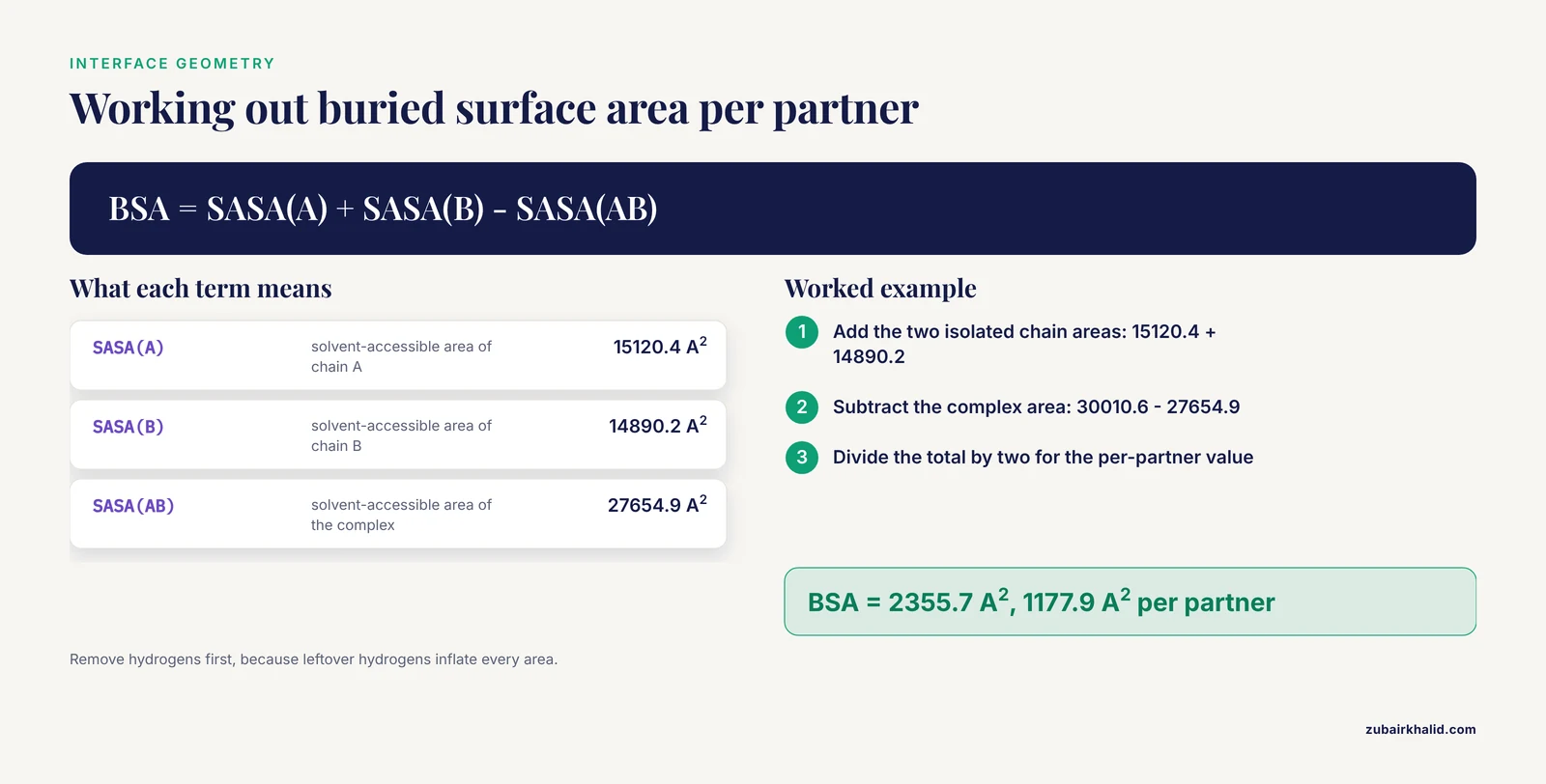
Confidence says how sure the network is. Geometry says whether the pose is physically sensible. Save this script and run it on the relaxed top model:
# pymol_bsa.py, run with: pymol -cq pymol_bsa.py
from pymol import cmd

cmd.set("dot_solvent", 1)
cmd.load("afm_out/complex_relaxed_rank_001_model_2_seed_001.pdb", "complex")
cmd.remove("hydrogens")
cmd.create("chainA", "complex and chain A")
cmd.create("chainB", "complex and chain B")
area_a = cmd.get_area("chainA")
area_b = cmd.get_area("chainB")
area_ab = cmd.get_area("complex")
bsa = area_a + area_b - area_ab
print(f"SASA A = {area_a:.1f} A^2")
print(f"SASA B = {area_b:.1f} A^2")
print(f"SASA AB = {area_ab:.1f} A^2")
print(f"Buried surface area = {bsa:.1f} A^2")
print(f"Per partner = {bsa/2:.1f} A^2")
Illustrative output:
SASA A = 15120.4 A^2
SASA B = 14890.2 A^2
SASA AB = 27654.9 A^2
Buried surface area = 2355.7 A^2
Per partner = 1177.9 A^2
The formula is the classic one: buried surface area equals the sum of the isolated chain solvent-accessible surface areas minus the area of the complex. Removing hydrogens first matters, because leftover hydrogens inflate every area. Interfaces of stable complexes commonly bury on the order of a thousand or more square angstroms per partner, while a hairline contact burying a few dozen square angstroms deserves suspicion regardless of ipTM.
Identify the interface residues and their interactions interactively in PyMOL:
load afm_out/complex_relaxed_rank_001_model_2_seed_001.pdb, complex
select ifaceA, chain A within 4 of chain B
select ifaceB, chain B within 4 of chain A
show sticks, ifaceA or ifaceB
distance hbonds, ifaceA, ifaceB, 3.5, mode=2
iterate ifaceA, print(resn + resi)
The two within 4 of selections define the interface as residues with any atom within 4 angstroms of the partner, a standard working definition. The distance command with mode=2 draws polar contacts within 3.5 angstroms, which gives you a hydrogen bond and salt bridge census. Record the counts. Then check for steric clashes with MolProbity:
phenix.molprobity afm_out/complex_relaxed_rank_001_model_2_seed_001.pdbA clashscore in the low single digits is comfortable. A double-digit clashscore on a high-ipTM model is a red flag that the pose is compressed and needs relaxation or refinement before any other interpretation.
If a Selector-Error: Invalid selection name appears, the select command defining that name has not run yet in the session. Execute the selections in order.
Step 5. Rescore With Independent Methods
Every metric in Step 3 came from the same network that produced the coordinates. Independent scoring closes that loop, and the CAPRI community has converged on exactly this pattern of combining energy-based scoring with model confidence. In the eighth CAPRI exercise, the pyDock team scored AlphaFold-Multimer models with a combination of pyDock interaction energy and AF model confidence [8], and their methods chapter walks through the practical recipe of generating diverse AlphaFold models and identifying the correct ones with the pyDock energy function [9].
Learned interface quality assessment tools add a second independent view. Three are worth knowing by name:
- TopoQA assesses interface accuracy using topological features captured by persistent homology inside a graph neural network, and it outperforms AF-Multimer-based AF2Rank on standard benchmark sets [10]
- EquiRank estimates interface quality with an equivariant graph neural network built on ESM-2 language model embeddings, and it improves ranking over the top CASP15 method VoroIF_GNN as well as over the AlphaFold-Multimer self-assessment repurposed for complex scoring [11]
- EuDockScore provides Euclidean graph neural network scoring of protein-protein interfaces, with a dedicated antibody-antigen variant called EuDockScore-Ab [12]
For pairs with sparse evolutionary signal, such as engineered proteins or cross-species complexes, contact prediction and rescoring methods built on geometric rather than coevolutionary features hold up better. ProTact, a physics-informed geometric network, delivers large precision gains on CASP and DIPS-Plus targets and improves on AlphaFold3's default confidence scores in low-MSA settings [13].
The practical rule: require agreement between at least two independent scores before you promote a model. If pyDock likes the pose and a learned QA method ranks it first, confidence rises. If they disagree, the model stays in the refine pile.
Step 6. Cross-Check With Docking and Orthogonal Evidence
Docking remains a genuinely useful control, not a legacy method. A systematic evaluation of eleven docking approaches across Docking Benchmark 5.5, a new antibody-antigen set, and an out-of-distribution set found that AlphaFold 3 reached a top-5 success rate of 77.98 percent docking against apo structures, while HDOCK managed only 12.84 percent on apo targets despite reaching 85.24 percent against holo structures [14]. The asymmetry teaches the right lesson: when you already have good individual structures, classical docking is a fast, independent check on whether the AF pose sits among the solutions a physics-aware sampler would find.
Hybrid pipelines formalize this. The ClusPro team at CASP16 combined FFT docking and molecular dynamics sampling with AlphaFold-based sampling and refinement, producing high-accuracy models for cases where AlphaFold alone failed [15]. Across CAPRI rounds 47 to 55, teams that integrated AlphaFold into their pipelines and then enhanced the sampling strategy around it improved their prediction accuracy in the later rounds [16]. For cases with expected conformational change on binding, where AlphaFold-Multimer struggles most, replica-exchange docking initialized from AF models is the designed remedy [1].
The protein-RNA benchmark behind the AlphaFold Server evaluation adds a nuance that generalizes: AlphaFold 3 achieved an overall top-5 success rate of 87.0 percent, yet it failed on nine complexes where the docking servers succeeded [6]. A cheap docking cross-check catches exactly those cases.
Orthogonal biological evidence turns a plausible model into a credible one:
- Map missense variants and disease mutations onto the interface. A structural interactome built from 1.5 million pairwise AlphaFold-Multimer predictions in Drosophila found phenotype-associated missense mutations enriched at predicted interfaces [17]
- Check conservation of interface residues across orthologs
- Overlay known motif annotations, especially for domain-motif candidates
- Design experiments. An AlphaFold 3 model of the monkeypox G9/A16/A56/K2 assembly predicted that the M142I substitution widens the interfacial gap and weakens docking stability, and ELISA binding assays confirmed the reduced affinity experimentally [18]
- For inhibitor-facing questions, a combined workflow of split-luciferase complementation, intrinsic fluorescence spectroscopy, and surface plasmon resonance was used to characterize and disrupt the GSK3β/Nav1.6 C-terminal interface, with AlphaFold modeling placing the compound binding site at the predicted interface [19]
Step 7. Decide and Document
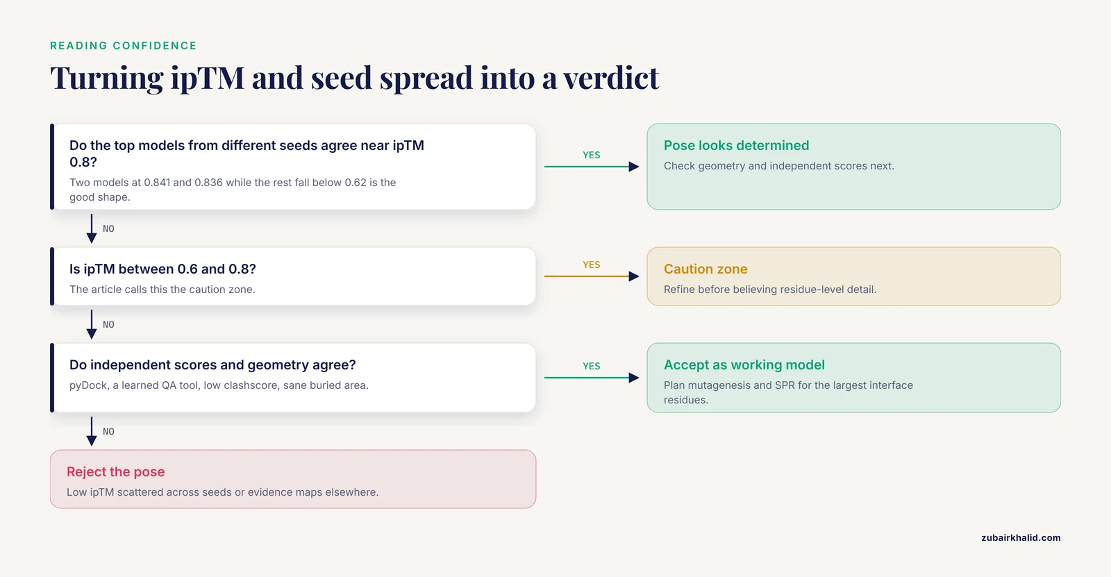
Convert everything into one of three verdicts:
- Accept as working model. ipTM at or above 0.8, stable pose across seeds, low cross-chain PAE, sane buried surface area, low clashscore, agreement between at least two independent scores, and no contradicting biological evidence.
- Refine. Moderate confidence or good confidence with physical problems. Route to energy-based rescoring, replica-exchange refinement, or molecular dynamics before believing the details.
- Reject. Low ipTM scattered across seeds, contradictory independent scores, or orthogonal evidence that maps elsewhere.
Then write the report. This is the template to reuse, and filling it takes about twenty minutes once the numbers exist:
# Interface validation report

## Prediction
- Sequences and isoforms used, with UniProt accessions
- Chain order and stoichiometry exactly as in the FASTA
- Software and versions (ColabFold release, alphafold2_multimer_v3)
- MSA mode, number of models, number of seeds, recycle count

## Confidence
- Table of ipTM, pTM, and mean pLDDT for every model and seed
- Median inter-chain PAE for the top model
- Mean pLDDT restricted to interface residues

## Geometry
- Buried surface area, total and per partner
- Interface residue counts per chain and total contact count
- Hydrogen bonds, salt bridges, hydrophobic contacts
- Clashscore

## Independent assessment
- pyDock energy score or equivalent, with comparison context
- Learned QA scores (TopoQA, EquiRank, EuDockScore)
- Docking cross-check (HDOCK, ClusPro, AlphaRED) and level of agreement

## Evidence
- Variants and mutations mapped to the interface
- Conservation, motif annotations, prior experimental results

## Decision
- Accept as working model / refine / reject
- Planned experiments (mutagenesis, SPR, pull-down, cell-based assay)
A Worked Example, Start to Finish
To make the whole loop concrete, suppose you predict a 287-residue kinase domain against a 214-residue regulatory protein. You run 15 predictions. The top two models, from different seeds, sit at ipTM 0.841 and 0.836 while the remaining thirteen fall below 0.62, so the pose is determined and reproducible. Median inter-chain PAE is 3.14 angstroms with 71 percent of cross-chain residue pairs below 5 angstroms. Buried surface area is 2356 square angstroms total, about 1178 per partner, with 26 interface residues per chain, 14 hydrogen bonds, and a hydrophobic core at the center of the patch. Clashscore is 8.4. pyDock ranks the model favorably, TopoQA places it first among the ensemble, and HDOCK sampled the same contact patch independently. Two known activating mutations map to the interface rather than to the catalytic site. Verdict: accept as a working model, and plan an alanine scan of the three largest interface residues followed by surface plasmon resonance against the wild-type interface peptide. Every number here is illustrative, but the decision logic is exactly what you should apply to your own runs.
Common Mistakes and Limitations
- Treating the rank as the truth. The internal ranking score weights confidence, not correctness, and the CAPRI record contains accurate models that ranked low and confident models that were wrong [7]. Always look past rank_001.
- Running one model and one seed. A single confident-looking prediction proves nothing about reproducibility. The ensemble spread is itself a result.
- Feeding full-length disordered chains and expecting domain-level answers. Long disordered regions depress confidence and blur interfaces, while aggressive trimming can manufacture contacts that do not survive full-length context. Fragmentation is a design decision, not a hack, and it changes both sensitivity and specificity [3].
- Ignoring distribution shift. Accuracy measured on benchmarks overstates accuracy on unfamiliar targets. On the LiPP lipid-protein benchmark, AlphaFold 3 succeeded on 76.1 percent of complexes overall but dropped to 47.2 percent for structures not seen during training [20]. Novel folds, engineered proteins, and unusual stoichiometries deserve extra scrutiny.
- Applying monomer intuition to antibodies. Antibody-antigen interfaces are a documented weak spot for AlphaFold-Multimer, and a high ipTM on an antibody complex deserves independent confirmation before any design decision [1].
- Getting stoichiometry wrong. A heterodimer predicted as two monomers, or a trimer predicted as a dimer, produces a confident model of the wrong assembly. Check known oligomeric states in UniProt annotations before running.
- Skipping relaxation and clash checks. Unrelaxed models can carry sterically implausible contacts that distort contact counts and buried area. Relax first, then measure.
- Overreading side-chain detail. Interface side-chain orientations are the least reliable layer of any prediction. Treat residue-level contacts as hypotheses for mutagenesis, not as measurements.
Frequently Asked Questions
How do you validate an AlphaFold-Multimer interface without a crystal structure?
Combine the four pillars: predictor confidence led by ipTM, physical interface geometry, independent rescoring and docking cross-checks, and orthogonal biological evidence. Promote to experimental validation only the candidates that pass all four.
What ipTM value is good enough?
The working rule of thumb is ipTM at or above about 0.8 for a trustworthy interface, 0.6 to 0.8 as a caution zone, and below 0.6 as unresolved. Treat the threshold as a filter, not a verdict, because confidently wrong poses exist.
Can I use the AlphaFold Server instead of installing anything?
Yes. The AlphaFold Server runs AlphaFold 3 from a browser and its models can be validated with this same checklist after converting the mmCIF output to PDB. It is rate-limited and does not accept custom MSAs or templates, which matters for unusual or confidential sequences.
How many models and seeds should I generate?
Run all five models per seed at minimum and repeat with at least three seeds. Fifteen predictions cost little and the spread across them is one of the most informative validation signals you will get.
Why does my full-length protein fail while a fragment works?
Long disordered regions degrade prediction quality and dilute interface signal. For domain-motif interactions, predicting a structured domain against a short motif peptide often works better than full-length against full-length, but fragments also raise false-positive risk, so validate both directions.
Which rescoring tool should I pick?
Start with an energy-based scorer such as pyDock combined with the model confidence, then add one learned interface quality assessment method such as TopoQA, EquiRank, or EuDockScore. Agreement between two independent scores is the goal.
What should a validation report contain?
Inputs and versions, the full metric table across models and seeds, interface geometry measurements, independent scores, orthogonal evidence, and an explicit accept, refine, or reject decision with planned experiments. The template in Step 7 covers all of it.
When should I abandon AlphaFold-Multimer for docking?
Complement or switch when you expect large conformational change on binding, when confidence stays low across all seeds, or when the target is an antibody-antigen pair where AlphaFold-Multimer historically struggles. Hybrid pipelines that dock around AF models exist for exactly these cases.
Sources
- Reliable protein-protein docking with AlphaFold, Rosetta, and replica exchange.
- Bias in, bias out - AlphaFold-Multimer and the structural complexity of protein interfaces.
- Systematic discovery of protein interaction interfaces using AlphaFold and experimental validation.
- Computational methods for modeling protein-protein interactions in the AI era: Current status and future directions.
- Improving protein and protein interactions using pseudo-dimers derived from monomeric proteins.
- Evaluation of protein-RNA Docking Web Servers for Template-Free Docking and Comparison with the AlphaFold Server.
- AlphaFold and Docking Approaches for Antibody-Antigen and Other Targets: Insights From CAPRI Rounds 47-55.
- Performance of pyDock in 8th CAPRI: Energy-Based Scoring Applied to Docking and AlphaFold Models.
- Modeling Protein-Protein Complexes by Combining pyDock and AlphaFold.
- TopoQA: a topological deep learning-based approach for protein complex structure interface quality assessment.
- EquiRank: Improved protein-protein interface quality estimation using protein language-model-informed equivariant graph neural networks.
- EuDockScore: Euclidean graph neural networks for scoring protein-protein interfaces.
- Accurate protein-protein interactions modeling through physics-informed geometric invariant learning.
- Revisiting Protein-Protein Docking: A Systematic Evaluation Framework.
- Modeling Protein-Protein and Protein-Ligand Interactions by the ClusPro Team in CASP16.
- Protein Complex Structure Prediction With AlphaFold-Enhanced HDOCK in CAPRI Rounds 47-55.
- FlyPredictome: A structural atlas of predicted protein-protein interactions in Drosophila.
- Structural Insights into the Impact of the M142I Mutation in Monkeypox Virus G9 Protein on Subcomplex Formation Revealed by AlphaFold 3 Modeling.
- Targeting the noncatalytic activity of GSK3β modulates neuronal excitability in medium spiny neurons via Nav1.6 interactions.
- The LiPP Benchmark Set for Modeling Lipid-Protein Complexes: Comparison of Co-Folding and Docking Methods.