How to Use UniProt to Prepare Your Protein Sequence for AlphaFold

By Dr. Zubair Khalid, DVM, MS, PhD · 2026-11-11

This guide provides a comprehensive, reproducible workflow for transforming protein sequence data obtained from UniProt into a format suitable for high-accuracy structural prediction using AlphaFold. Whether you are running predictions on a local instance, utilizing an official AlphaFold server, or preparing data for downstream structural analysis, the quality and preparation of your input sequence are paramount to achieving reliable results.

By the end of this guide, you will be able to:

Identify and retrieve relevant protein sequences and metadata from UniProt.
Perform essential sequence cleaning and formatting required for AlphaFold input.
Execute AlphaFold predictions using various computational platforms.
Validate and interpret the structural output against UniProt annotations.

Prerequisites and Setup

Before beginning the sequence preparation process, ensure you have the necessary software and data access.

Required Tools and Access:

UniProt Account: Access to the UniProt database is required for sequence retrieval.
Sequence Editor: A text editor capable of handling FASTA format (e.g., VS Code, Sublime Text).
Computational Environment:
For Server Use: Access to an AlphaFold server (e.g., official Google DeepMind servers, or community-maintained instances).
For Local Use: A robust GPU environment with the necessary dependencies for running AlphaFold locally.
Bioinformatics Tools: Command line access to tools like grep, awk, and potentially specialized pipelines like ProtPen, which integrates sequence and structural predictions [1].

Phase 1: Retrieving Sequences from UniProt

UniProt serves as the primary source for protein sequences and associated biological annotations. The first step in the UniProt to AlphaFold sequence workflow is identifying and extracting the correct sequence.

1.1 Identifying Target Proteins

Identify the specific protein(s) of interest. You should use stable identifiers such as the UniProt Accession ID (e.g., P12345) or the protein name.

1.2 Sequence Retrieval Methods

There are several methods to retrieve sequences from UniProt.

A. Manual Retrieval: Navigate to the UniProt website, search for the accession ID, and copy the primary sequence from the "FASTA" tab. This method is suitable for single protein analysis.

B. Automated Retrieval (Recommended): For batch processing, use the UniProt API or the wget command targeting the UniProt FTP site. This is the most efficient method for large proteome-scale studies.

# Example: Downloading sequences for a list of UniProt IDs
# Replace 'ID1,ID2,ID3' with your actual list of UniProt accessions.

# Use a list file containing one ID per line
cat list_of_uniprot_ids.txt | xargs -L 1 wget -O uni_seq.fasta "https://www.uniprot.org/uniprot/fasta/UniProtKB/[ID]"

Note: This command assumes you have a text file named list_of_uniprot_ids.txt where each line is a UniProt accession ID.

Phase 2: Sequence Preparation and Formatting

AlphaFold requires a specific input format, typically a FASTA file containing only the amino acid sequence, free of extraneous metadata.

2.1 Cleaning the Sequence

UniProt entries often contain multiple isoforms or splice variants. If your goal is structural prediction, you must select the most representative sequence.

Selecting the Canonical Sequence: For most structural predictions, use the canonical (full-length) sequence provided by UniProt, unless you are specifically studying a known splice variant or truncated form [2].
Filtering: Use command-line tools to ensure the FASTA file contains only the sequence and the header.

# Example: Extracting only the sequence from a potentially messy UniProt download
awk '/^>/ {print; next} /^[A-Z]+$/ {print}' uni_seq.fasta > clean_input.fasta

2.2 Handling Sequence Length and Truncation

AlphaFold models have input limits. While modern versions of AlphaFold can handle long sequences, very long proteins may require domain decomposition.

Domain Decomposition: If a protein is extremely large, consider using domain prediction tools (like Pfam or InterPro) to break the protein into functional domains. Predicting domains separately and then assembling the structures is a common strategy in structural biology [3].
Domain Trimming: If you are studying a specific interaction, you may need to trim the sequence to the interacting domain. However, be cautious. Trimming can affect the predicted structure of the full protein, which is crucial for accurate modeling of the entire chain. If you trim, you must account for this in downstream analysis, especially when calculating metrics like ipTM (Interface Prediction Score) [4].

2.3 Sequence Validation (Self-Check)

Before running a computationally intensive prediction, verify the sequence integrity.

Residue Consistency: Check the sequence against known structural databases like the Protein Data Bank (PDB) if a structure already exists. Tools like 3DSeqCheck allow for verifying sequence consistency between a known 3D structure and its corresponding UniProt entry [5].
Quality Assessment: For sequences derived from experimental data, ensure they are free of ambiguous residues (e.g., 'X' or gaps) unless those gaps are intentional for a specific study, such as analyzing disordered regions [6].

Phase 3: Executing the AlphaFold Prediction Workflow

The method you use to run AlphaFold depends on your computational resources and scale of analysis.

3.1 Using the AlphaFold Server (Recommended for Beginners)

The AlphaFold server is the most straightforward way to begin an AlphaFold tutorial. It is hosted by major research institutions and provides an easy interface for sequence submission.

Workflow Steps:

Obtain a sequence in FASTA format (e.g., clean_input.fasta).
Navigate to the chosen AlphaFold server interface.
Upload the FASTA file or paste the sequence.
Submit the job. The server will run the prediction and generate a set of output files, typically including the PDB structure and the confidence metrics (pLDDT and PAE).

Tip: When using a server, always check the service's current queue time and recommended input file size limits.

3.2 Local Installation and API (Recommended for Production Pipelines)

For high-throughput structural biology, running AlphaFold locally or via a dedicated API is necessary.

A. Local Installation: Install the required environment (e.g., using Docker or Conda) and run the prediction using the local AlphaFold binaries.

# Example: Running AlphaFold locally (requires specific hardware and setup)
alphafold run clean_input.fasta

B. API Integration: If you are integrating this into a larger pipeline (e.g., for function prediction using ProtPen), you may use an API that accepts UniProt identifiers directly. ProtPen, for example, requires only a FASTA file containing UniProt identifiers for its pipeline [1].

Phase 4: Interpreting and Utilizing the Output

Once the prediction is complete, the output files contain the 3D coordinates (PDB format) and quality metrics.

4.1 Assessing Prediction Confidence

The quality of the prediction is not uniform. Always check the following metrics:

pLDDT (Predicted Local Distance Difference Test): This score (ranging from 0 to 100) indicates the confidence in the prediction of each residue. Scores above 90 generally indicate high confidence in the local structure.
PAE (Predicted Aligned Error): This metric estimates the uncertainty in the position of each residue. Lower PAE values indicate higher structural certainty.

4.2 Retrieving Structures via UniProt Accessions (Advanced Workflow)

If you only need the structure for a protein you already have a UniProt ID for, you can bypass the prediction step and retrieve existing predicted or experimental structures.

The AlphaFold Database Structure Extractor is a tool that allows you to download structures using standard identifiers, including UniProt accessions [7].

# Example: Using the AlphaFoldDB Structure Extractor (API or web interface)
# Input: UniProt Accession ID
# Output: PDB or mmCIF file
# Tool: AlphaFoldDB Structure Extractor

This method is particularly useful for mapping structural coverage across large proteomes, as the AlphaFold Protein Structure Database (AFDB) contains hundreds of millions of predictions [8].

Summary Table of Workflow Options

Step	Goal	Input	Output	Recommended Tool/Method	Key Consideration
1. Acquisition	Get sequence data.	UniProt Accession ID	FASTA Sequence File	UniProt API / `wget`	Ensure correct isoform selection.
2. Preparation	Clean and format sequence.	Raw FASTA	Clean FASTA Input	`awk` / Text Editor	Remove gaps or ambiguous residues if necessary.
3. Prediction	Generate 3D structure.	Clean FASTA	PDB/mmCIF Structure File	AlphaFold Server / Local Run	Check queue time and resource requirements.
4. Validation	Verify structure quality.	PDB + UniProt ID	Quality Report	3DSeqCheck / pLDDT Analysis	Compare sequence consistency with UniProt [5].

Common Mistakes and Limitations

Adhering to best practices minimizes errors in structural biology. Avoid these common pitfalls:

Using Incomplete Sequences: Submitting truncated sequences without clear justification can lead to misleading structural results. While domain decomposition is an option, it requires careful assembly and validation.
Ignoring Quality Metrics: Relying solely on the presence of a PDB file without checking pLDDT or PAE is a major mistake. A structure with low confidence metrics is not a reliable scientific result.
Misinterpreting ipTM Scores: When analyzing protein-protein interactions (PPI), be aware that the ipTM score can be misleading if the full-length sequence is used, especially if the chains contain large amounts of disordered or accessory domains that do not participate in the interaction [4].
Assuming Uniform Coverage: Not all organisms or protein classes are equally represented in the AlphaFold Database. For example, there is a substantial disparity in structural coverage between mammalian proteomes and those of plants [9].
Sequence Drift: UniProt entries are updated frequently. If you are using a structure predicted in 2024, ensure the underlying UniProt sequence annotation is current, as revisions can occur over time [5].

Reading a UniProt Entry Like a Structural Biologist

Before you touch a single command line tool, you need to understand what a UniProt entry actually contains, because most preparation errors trace back to misreading the entry page rather than to any technical failure downstream. A UniProt entry is not just a sequence. It is a curated bundle of annotations, and several of them directly affect how you should prepare your AlphaFold input.

When you land on an entry page after searching for your accession, focus on these regions:

Sequence section. This shows the full amino acid sequence with position numbering. Note the sequence version (for example, "Sequence version 3"). This matters because UniProt entries are revised over time, and a prediction made against an older sequence version may no longer match the current entry [5]. Record the sequence version in your lab notebook or pipeline metadata every time you download.

Isoform section. Many entries carry more than one isoform. The canonical sequence is the one UniProt considers the most prevalent, most conserved, or best supported representative [2]. Isoform sequences are listed separately, often with descriptions like "Isoform 2" and a short note describing how it differs from the canonical form (for example, a missing exon segment). If you predict a structure for the wrong isoform, every downstream comparison against literature structures or domain boundaries will be offset.

Features table. This is where structural biologists should spend the most time. The features table tells you:

Signal peptide ranges: residues expected to be cleaved during secretion. A mature secreted protein structure will not include the signal peptide, and including it in your AlphaFold input can distort the prediction of the N-terminal fold.
Chain and peptide ranges: the processed, mature form of the protein after cleavage.
Domain and region annotations: recurring modules, zinc fingers, coiled coils, and similar entries that help you decide whether domain decomposition is necessary.
Disordered region annotations: stretches annotated as lacking a fixed structure. These are the regions where AlphaFold confidence will typically collapse, and knowing their boundaries before you predict saves you from misinterpreting low confidence later [6].
Variants: disease-associated or polymorphic residue changes. If you plan to model a variant protein, you need the wild-type numbering scheme from this table to label your mutation correctly.

Cross-references. The PDB cross-references list experimental structures. Always check this before running a prediction. If a high-quality experimental structure exists, your prediction may be redundant, or at minimum you should plan to compare your model against the experimental coordinates. Tools such as 3DSeqCheck exist precisely to verify that a structural model and its UniProt counterpart describe the same sequence [5].

Taxonomy and gene ontology. Less obvious but useful: knowing the organism lets you sanity-check the sequence length against paralogs. A common silent failure is retrieving a sequence from the wrong ortholog because two entries share nearly identical gene names.

A practical habit: before downloading anything, screenshot or export the entry page, or use UniProt's own text export to capture the features table. You will want those residue ranges later when you map your predicted structure back onto known biology.

Choosing Between Canonical, Isoform, and Custom Sequences

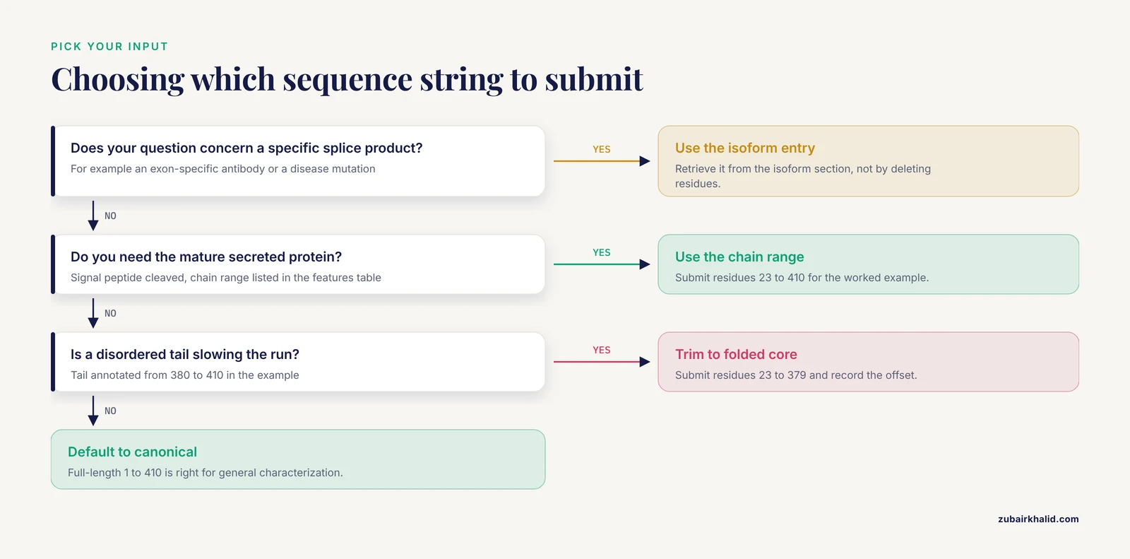
Decision path asking whether the question concerns the mature protein, an isoform, or the full precursor, ending in the recommended input sequence.

The single most consequential decision in the UniProt to AlphaFold sequence workflow is which amino acid string you submit. There are three legitimate choices, and each answers a different scientific question.

Canonical sequence. Use this as your default. UniProt defines the canonical sequence as the most representative form, and for general structural characterization it is almost always the right input [2]. When you publish a model built from the canonical sequence, other researchers can reproduce your work by citing the accession alone.

Isoform sequence. Use this when your experiment, your antibody, or your disease mutation maps to a specific splice product. Isoform-specific structural differences can be dramatic: an alternatively spliced exon may remove an entire interaction surface. In that case, predicting the canonical structure would be actively misleading, and the isoform sequence is the correct input. Retrieve isoform sequences from the entry's isoform section, not by manually deleting residues from the canonical sequence, because UniProt isoform entries carry their own identifiers that make your work traceable.

Custom constructed sequence. Use this when you are modeling a mature processed protein, a engineered construct, or a specific truncated domain. This is where discipline matters most, and it connects directly to the ipTM caveat discussed earlier in this guide: if you trim a sequence to an interaction domain, you must interpret interface scores in light of that trimming, because the context of the full-length chain changes the confidence profile [4].

A worked decision example. Suppose your protein of interest is annotated with a signal peptide spanning residues 1 to 22, a mature chain from 23 to 410, and a C-terminal disordered tail from 380 to 410. Three defensible inputs exist:

Full canonical sequence (1 to 410). Correct if you want the full-length picture, including how the disordered tail relates to the folded core, accepting that the tail region will show low pLDDT.
Mature chain only (23 to 410). Correct if you are comparing against an experimental crystal structure of the secreted protein, since crystals of secreted proteins nearly always begin after signal peptide cleavage.
Folded core only (23 to 379). Correct if the disordered tail is causing the whole prediction to run slowly or if you are modeling a complex with a partner and want to reduce noise.

Whichever you choose, document it. A one-line note such as "predicted UniProt P12345 canonical, residues 23 to 410, signal peptide removed per features table" is the difference between a reproducible analysis and an untraceable PDB file.

One frequent misconception deserves explicit correction: deleting residues from a UniProt sequence does not produce an isoform. Real isoforms can include residue substitutions and insertions, not just deletions, so manual editing of the canonical string is not equivalent to using the annotated isoform sequence [2].

A Robust Batch Retrieval Workflow for UniProt Sequences

The retrieval snippet shown earlier in this guide works for quick jobs, but production work benefits from a sturdier pattern. The issues with naive one-by-one downloads are familiar to anyone who has run them: failed transfers leave empty or truncated files, sequential requests are slow for hundreds of accessions, and nothing in the output tells you which accession a broken file came from.

Here is a batch workflow that addresses those failure modes using the same UniProt FASTA endpoint referenced earlier, wrapping each download in verification.

Step 1: Prepare a clean ID list.

# Strip whitespace and blank lines from your accession list
sed 's/[[:space:]]//g' raw_ids.txt | grep -v '^$' > list_of_uniprot_ids.txt

Sanity check the format. UniProt accessions are six or ten characters, typically letters followed by digits and then letters and digits. A quick filter catches spreadsheet artifacts:

# Show any lines that do not look like accessions
grep -vE '^[A-Z0-9]{6}([A-Z0-9]{4})?$' list_of_uniprot_ids.txt

If this prints anything, fix your list before proceeding. Duplicated accession columns from a copied spreadsheet are the most common contaminant.

Step 2: Download with per-file naming and size verification.

while read ACC; do
  outfile="fasta/${ACC}.fasta"
  wget -q -O "$outfile" "https://www.uniprot.org/uniprot/fasta/UniProtKB/${ACC}"
  # A valid FASTA has a header line starting with > and at least some sequence
  if ! grep -q '^>' "$outfile" || [ ! -s "$outfile" ]; then
    echo "FAILED: $ACC" >> download_failures.txt
    rm -f "$outfile"
  fi
done < list_of_uniprot_ids.txt

This loop writes each sequence to its own named file, which makes debugging far easier than one concatenated file, and it logs failures to a separate report rather than letting them fail silently.

Step 3: Validate residue content across the whole batch.

# Flag any downloaded sequence containing characters outside the standard
# amino acid alphabet (this permits X, B, Z, U and O, which you will review manually)
for f in fasta/*.fasta; do
  bad=$(grep -v '^>' "$f" | grep -c '[^ABCDEFGHIKLMNPQRSTVWXYZUO]')
  if [ "$bad" -gt 0 ]; then
    echo "Non-standard characters in $f"
  fi
done

Step 4: Concatenate the clean files into one working FASTA.

cat fasta/*.fasta > all_targets_raw.fasta

Step 5: Log your retrieval date and UniProt sequence versions. Because UniProt entries are revised over time, a prediction made this year may silently diverge from the entry next year [5]. The simplest reproducibility practice is to record the retrieval date alongside each accession in a small tab separated metadata file. If a reviewer or collaborator re-runs your workflow two years later and 3DSeqCheck flags a mismatch between your model and the current UniProt entry, your log will explain it [5].

For proteome-scale studies, where you need every protein from an organism rather than a hand-picked list, batch retrieval through the UniProt API in tabular or FASTA form is the appropriate route, and the per-file verification logic above still applies.

Validating and Sanitizing FASTA Files Before Prediction

The cleaning step deserves more depth than a single awk one-liner, because FASTA files accumulate more varieties of cruft than most people expect. Here is a systematic validation pass you can run on any file before submission.

Check the header line. A well-formed FASTA header starts with a greater-than symbol and contains no spaces in the identifier portion. UniProt FASTA headers are usually well behaved, but files that passed through spreadsheets, email clients, or manual copy paste frequently lose the leading > or gain smart quotes. A prediction server may reject such a file outright or, worse, silently treat garbage as sequence.

# Confirm every sequence block is preceded by a header
grep -c '^>' all_targets_raw.fasta

Compare that count against the number of accessions you requested. A mismatch means duplicated or missing headers.

Check the alphabet. The twenty standard amino acids are the safe alphabet for AlphaFold input. Beyond them:

X means an unknown residue. UniProt sequences contain X at positions of uncertain sequencing, and leaving them in can degrade a prediction or be rejected outright [6].
B (aspartic acid or asparagine), Z (glutamic acid or glutamine), and J (leucine or isoleucine) are ambiguity codes. Decide per case whether to resolve them or trim them.
U (selenocysteine) and O (pyrrolysine) are rare and should trigger a manual review of the entry.
**Asterisk ()*: a stop codon marker. This must never reach a prediction. It usually indicates you copied a translated nucleotide sequence rather than a curated protein sequence.
Gaps or dashes: these belong in alignments, not in a prediction input. Strip them.

Normalize letter case. Some sources emit lowercase sequence, which is legal FASTA but can confuse validation scripts and some web forms:

awk '/^>/ {print; next} {print toupper}' input.fasta > upper.fasta

Remove line length irregularities. Sequence lines of wildly inconsistent length are harmless to most tools but make visual inspection and positional arithmetic error prone. Rewrapping to a fixed width is a courtesy to your future self.

Verify expected length. Compare the sequence length in your FASTA against the length stated on the UniProt entry page. This single check catches the majority of copy paste disasters, including isoform mix-ups, because the entry page lists the length of each sequence variant explicitly.

Ambiguity as a signal, not just noise. A sequence dense with X residues is not automatically bad. Regions of unresolved sequence often correspond to poorly characterized or repetitive stretches. Cross-check where the X residues fall against the disordered region annotations in the UniProt features table [6]. If ambiguity clusters inside a region you plan to ignore anyway, trimming may be justified. If it falls inside a domain you care about, resolve the ambiguity before predicting, or at minimum annotate it in your results.

Working With Signal Peptides, Transit Peptides, and Processing Annotations

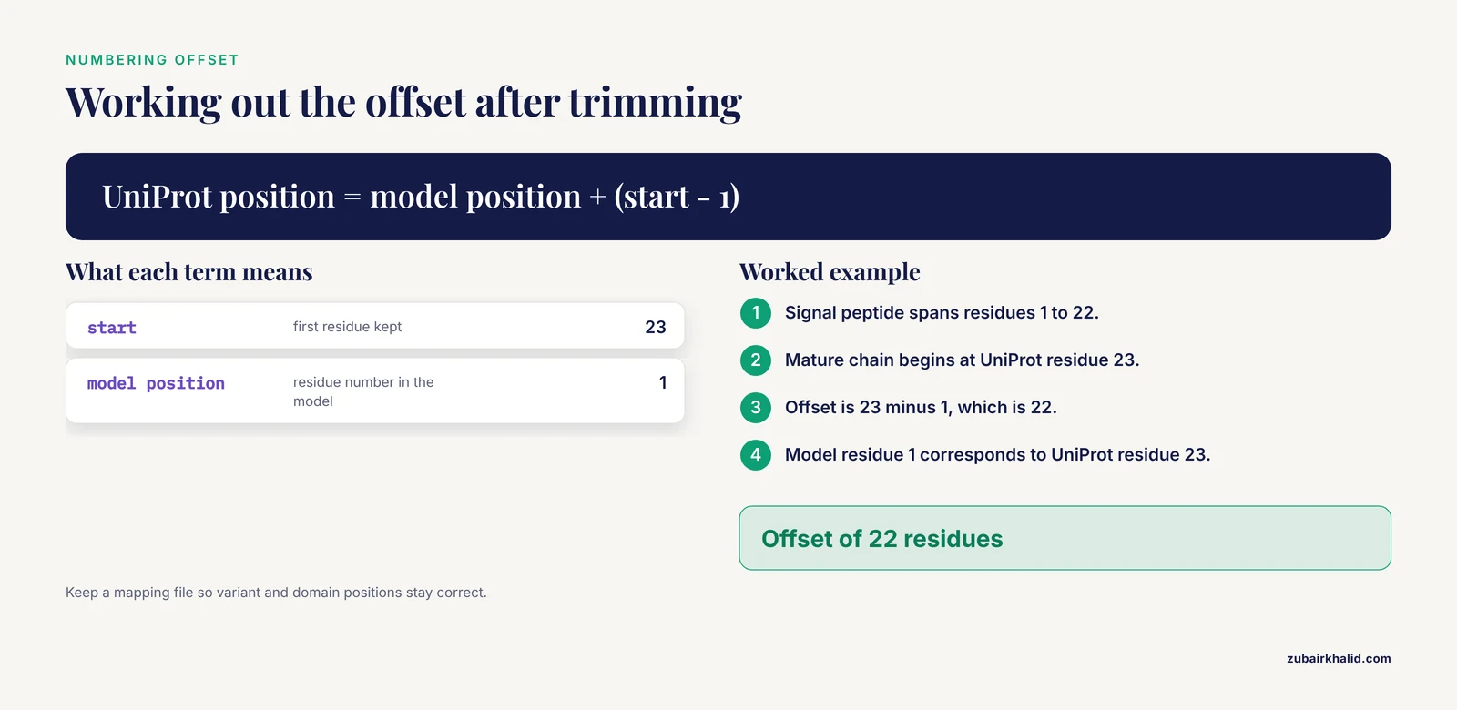
Calculation showing that a mature chain starting at UniProt residue 23 appears as residue 1, so UniProt position equals model position plus 22.

One class of UniProt annotation causes more avoidable confusion in AlphaFold work than any other: co-translational and post-translational processing features. Understanding them changes what you submit and how you interpret the output.

Signal peptides. A signal peptide is an N-terminal targeting sequence that is cleaved off as the protein crosses the membrane. Structurally, signal peptides are helical segments embedded in the secretion machinery, not part of the mature folded protein. Two problems arise if you leave them in your input:

The predicted model will include a helix that is not present in the mature protein, shifting your residue numbering by the length of the signal peptide relative to every experimental structure of the mature form.
The confidence profile at the N-terminus may reflect a transient, membrane-associated state rather than the soluble mature fold.

The right input for a mature secreted protein is the chain range listed in the UniProt features table, which begins after the signal peptide cleavage site. Extract it with an offset-aware command. For example, to keep residues 23 to the end:

# Keep header, then slice sequence from position 23 onward
awk '/^>/ {print; next} {print substr($0, 23)}' full.fasta > mature.fasta

Transit peptides and propeptides. Mitochondrial transit peptides and propeptides follow the same logic: annotated as cleaved, therefore absent from the mature functional structure. Treat them the same way as signal peptides when your scientific question concerns the mature protein.

When to keep the full-length precursor. Sometimes the precursor is exactly what you want. If you are studying the mechanism of processing itself, or modeling a biosynthetic enzyme whose domains are separated by cleavable segments, the full-length sequence is the correct input. The rule is simple: let your biological question dictate the construct, and let the UniProt features table supply the coordinates.

Numbering discipline. Every time you trim, your predicted structure's residue numbering no longer matches UniProt numbering. The mature chain that begins at UniProt residue 23 will appear as residue 1 in the trimmed prediction. This is the root cause of countless off-by-22 errors when researchers map a predicted structure back onto variant annotations or domain boundaries. Either renumber your model back to UniProt coordinates using the offset you applied, or maintain a mapping file alongside the model. The same discipline matters when comparing against PDB entries, where authors frequently use their own numbering schemes, and it is one more reason to verify consistency between a structural model and its UniProt source with a dedicated check rather than by eye [5].

Handling Intrinsically Disordered Regions in Your Input

Intrinsically disordered regions deserve their own section because they sit at the intersection of sequence preparation and honest interpretation.

UniProt annotates disordered regions in the features table, and these annotations are worth reading before every prediction. When you submit a protein containing large disordered stretches, two things happen. First, the prediction will typically assign those residues low pLDDT and elevated PAE, which is the correct behavior: the model is telling you it has no stable structure to offer there [6]. Second, long disordered tails increase computation time and, on some platforms, consume a large share of your allowed input length for information that will not yield a structure.

This creates a genuine decision point, not a rule. Consider these scenarios:

Your question concerns the folded domain. Trim the disordered tail. The prediction will be faster and your confidence summary will reflect the part you care about. Record the trimming explicitly, and remember the downstream accounting requirement for interaction scores mentioned earlier in this guide [4].
Your question is whether the tail is disordered. Keep it, and treat the low confidence region as positive evidence consistent with the UniProt disorder annotation [6]. Low pLDDT on an annotated disordered region is not a failure of the prediction; it is a confirmation.
Your question involves a binding region embedded in disorder. This is the hardest case. Some disordered segments fold upon binding. AlphaFold may or may not capture this depending on context, and a low confidence stretch does not prove the absence of an inducible fold. Report it as unresolved rather than as unstructured.

A practical trap to avoid: do not use low confidence disordered regions as an argument that the whole prediction is bad. Confident core domains and floppy termini routinely coexist in the same model. The correct reading is residue by residue, and the correct description in a paper is "the globular core was predicted with high confidence while the N-terminal 90 residues, annotated as disordered in UniProt, showed low confidence consistent with intrinsic disorder" [6].

Finally, note that ambiguous residues such as X often cluster in the same low complexity stretches that are disordered, so the ambiguity cleanup described in the validation section and the disorder considerations here frequently apply to the same region [6]. Resolving both in one pass, with one documented decision, keeps your workflow tidy.

Domain Decomposition in Practice: A Worked Example

Domain decomposition was introduced earlier as a strategy for very large proteins. Here is a concrete walkthrough of how to execute it defensibly, since "break the protein into domains" glosses over several decisions that determine whether the final assembly means anything.

Step 1: Identify domain boundaries from evidence, not convenience. Start with the domain and region annotations in the UniProt features table, then cross-check against Pfam or InterPro, both of which are reachable through the cross-references on the entry page. Look for boundaries that fall in annotated linker regions or disordered segments rather than cutting through a annotated domain. A boundary placed in the middle of a fold will produce a fragment that predicts poorly and assembles worse.

Step 2: Decide on overlap. A common practical choice is to include a modest overlap of linker sequence on each side of a domain so that the predictor has flanking context. There is no universal overlap length that suits every protein; the honest approach is to try the annotated boundary and one or two nearby alternatives and compare confidence metrics.

Step 3: Generate fragment FASTA files with tracked coordinates.

# Extract domain 1: residues 1 to 245 of the canonical sequence
awk '/^>/ {print; next} {print substr($0, 1, 245)}' full.fasta > domain1.fasta

# Extract domain 2: residues 246 to 610, renamed to start at 1
awk '/^>/ {print; next} {print substr($0, 246)}' full.fasta > domain2.fasta

Immediately write a mapping file recording that domain2 residue 1 corresponds to full-length residue 246. This file is your defense against the numbering chaos described earlier.

Step 4: Predict each fragment separately using your chosen AlphaFold server or local installation, and inspect pLDDT and PAE per fragment. A fragment whose confidence is dramatically worse than the same region predicted in the full-length context is telling you the boundary was wrong or that the domain depends on a distant segment for its fold. Iterate.

Step 5: Assemble with validation. Joining fragments into a composite model is where error accumulates, and it must be followed by validation rather than assumed. The earlier discussion of domain decomposition as a common strategy in structural biology comes with the corresponding warning that assembly requires careful validation [3]. Concretely: check that the assembled model's geometry is continuous across junctions, that interface regions between fragments show plausible packing, and that the assembled construct, when re-checked against the current UniProt entry, remains sequence consistent [5].

When not to decompose. If the full-length protein predicts within your platform's limits with acceptable confidence, predicting it whole is simpler and avoids the assembly problem entirely. Decomposition is a remedy for a specific constraint, not a default habit. And when decomposition is used because you are studying a specific interaction, remember the ipTM interpretation caveat: interface scores computed on trimmed constructs must be understood in that context [4].

AlphaFold Server Submission: A Detailed Walkthrough

The earlier section on using an AlphaFold server gave the outline. Here is a granular walkthrough of the submission process as it applies across the commonly used hosted interfaces, including the official Google DeepMind servers and community-maintained instances, since the mechanics are broadly similar even where the interfaces differ.

Before you touch the form: prepare the exact input. Have your cleaned FASTA file open and verified. Many researchers keep a dedicated submissions/ directory with one FASTA per prediction and a log file, so that every submission is traceable to a file that still exists months later.

Step 1: Confirm account and eligibility requirements. Hosted servers typically require an account and may impose terms on how results are used. Read these once, before your first submission, not after.

Step 2: Check the current queue and limits. As noted earlier, always check the service's current queue time and recommended input file size limits before committing to a server run. A queue measured in hours is fine for a single protein and unacceptable for a batch of fifty, which is the signal to move to local execution or an API route.

Step 3: Paste or upload the sequence. When pasting directly into a web form, watch for two classic failures: line breaks inserted by the browser at odd positions, and truncation of long sequences by clipboard limits. Uploading the file avoids both. After pasting, visually confirm the first and last ten residues against your file.

Step 4: Verify residue count. Many interfaces display a character count after entry. Compare it with the length you validated earlier. This ten-second check prevents the most embarrassing category of error: a perfectly executed prediction of the wrong sequence.

Step 5: Specify multiple chains if applicable. If you are predicting a complex, servers that accept multiple chains expect each chain in its own FASTA block with its own header. Do not concatenate two proteins into one continuous sequence to fake a complex; that produces a covalent linkage that does not exist biologically and will distort both the interface geometry and any interaction confidence scores you plan to report.

Step 6: Submit and record the job identifier. Save the job identifier or URL in your log immediately. Server-side job histories expire, and a prediction you cannot retrieve is a prediction you did not make.

Step 7: Download the complete output set. Do not stop at the structure file. Download the confidence metrics alongside the coordinates, because the PDB or mmCIF file without pLDDT and PAE is half a result. The interpretation of these files is covered in its own section below.

Step 8: Archive inputs and outputs together. A prediction is reproducible only if the exact input sequence, the submission date, and the platform are recorded. Store the input FASTA, the output archive, and a one-line provenance note in the same folder.

For researchers planning to hand their sequences to broader automated pipelines rather than a single interactive submission, integration frameworks that accept FASTA input with UniProt identifiers, such as the ProtPen pipeline combining sequence annotation with structural similarity search, offer a bridge between one-off server use and fully scripted production work [1].

Server Versus Local: Choosing the Right Execution Path

The existing guide states that servers suit beginners and local installs suit production. The decision deserves a fuller treatment because the tradeoffs are multidimensional and the wrong choice wastes either days of compute setup or days of queue time.

Choose an AlphaFold server when:

You have a small number of predictions, on the order of a handful to a few dozen.
Your sequences fall comfortably within the platform's input limits without decomposition.
You need results on a human timescale without installing anything.
You want the platform's curated output format, which simplifies downstream interpretation.
Your institution provides access to official or community-maintained instances and your data is not restricted.

Choose local execution when:

You run recurring predictions as part of a pipeline, for example nightly updates feeding a function annotation workflow [1].
You need to predict constructs, mutants, or trimmed domains in high volume, where server queues and per-submission overhead dominate.
Your data cannot leave your environment.
You need to control the exact software version for reproducibility, which matters because a model generated with a different version may not be comparable to your earlier results.

The hybrid pattern most groups converge on. Use the server interactively while you are still deciding on constructs: canonical versus trimmed, full-length versus decomposed. Once the construct decisions stabilize, script the finalized inputs for local execution or API submission. This mirrors the way the pipeline tools cited in this guide operate, accepting FASTA files with UniProt identifiers and running the sequence and structure stages automatically [1].

Resource reality check for local runs. The earlier guide notes that local use requires a robust GPU environment with the necessary dependencies. Plan for the setup cost honestly: containerized environments reduce installation pain, and databases required for sequence search dominate storage requirements. If your local hardware cannot accommodate the full pipeline, several reduced-database configurations trade some accuracy for feasibility, but any such trade must be documented because it affects confidence calibration.

A comparison summary without a table: server routes buy convenience, curated outputs, and zero setup at the cost of queue dependence, limited batch scale, and platform-imposed input limits. Local routes buy control, throughput, and version pinning at the cost of setup, maintenance, and hardware. Neither is universally correct, and the summary table earlier in this guide remains a useful map of where each step happens regardless of route.

Understanding Every File in an AlphaFold Output Directory

Interpreting output was introduced earlier with pLDDT and PAE. A complete prediction generates a richer set of files, and knowing what each one is for turns the output from a folder of mysteries into a working dataset.

The structure file (PDB or mmCIF). The atomic coordinates. The B-factor column in these files is repurposed to carry the per-residue pLDDT value, which is why structure viewers color AlphaFold models by confidence automatically. This is the single most useful piece of integration between the coordinates and the confidence metrics: open the structure, colored by pLDDT, and immediately see which regions to trust.

pLDDT per residue. As established earlier, scores above 90 indicate high confidence in the local structure. The full interpretive frame is worth restating in expanded form: high pLDDT means the local backbone geometry is confidently predicted, not that the residue's position relative to distant parts of the protein is equally certain. A helix can be individually confident while its orientation relative to another domain is not, which is precisely what PAE describes.

PAE matrix. The predicted aligned error is delivered as a matrix over residue pairs. Reading it is a skill worth building:

Dark blocks along the diagonal correspond to well-determined domains.
Dark blocks off the diagonal indicate confidently specified relative positions between two regions, which is how you recognize a predicted domain interface.
Light blocks between domains mean the relative arrangement of those domains is uncertain. This is the visual signature of a flexible multidomain protein, and it is the correct context for interpreting any single representative conformation as one sample from a distribution rather than a unique answer.

Per-residue confidence files. Many outputs include the raw per-residue confidence values in a separate file, which is what you use for scripted analyses, for example plotting confidence along the sequence and overlaying it against the UniProt feature track [6].

MSA and template evidence files. Depending on the platform, the output may include evidence about how many homologous sequences and structural templates informed the prediction. Low evidence depth is a common explanation for low confidence in otherwise normal-looking proteins, and checking it is the first diagnostic step when a prediction disappoints.

ranked output files. Where multiple structure hypotheses are generated, ranked files order them by overall confidence. For a single-chain monomer prediction the top-ranked model is typically the one you use, but inspecting alternatives is informative when the top ranks have similar scores.

A note on interpretation discipline: the earlier guide's warning against relying on the presence of a PDB file without checking metrics bears repeating in operational terms. The habit to build is that no model leaves your hands, internally or publicly, without a stated confidence summary: median pLDDT, the fraction of residues above the high-confidence threshold, and a one-sentence PAE characterization.

Mapping Predictions Back to UniProt Feature Annotations

A predicted structure becomes scientifically useful when its residues are connected back to the annotations that motivated the prediction. This mapping step is where the UniProt features table you captured early in the workflow pays off.

Overlay the feature track. For each annotated feature in the UniProt entry, such as an active site, a binding region, a domain, or a disordered segment, ask where it sits in the model and what the local confidence is. A binding site predicted with high confidence is a usable hypothesis for mutagenesis or docking. A binding site inside a low-confidence stretch is a caution flag, not a target.

Check variant positions. For entries with disease or polymorphism variants, map each variant residue into the model and record its pLDDT and local environment. A variant at a confidently buried core position suggests a stability hypothesis; the same variant on a disordered surface suggests a different, weaker interpretation. This single exercise converts a structure prediction into testable biology.

Verify sequence consistency as a final gate. Before any cross-referencing between a structural model and UniProt annotations, confirm that the sequence underlying the model matches the current UniProt entry. Dedicated tools such as 3DSeqCheck perform exactly this comparison between a structural model and its UniProt source [5], and given that UniProt entries are revised over time, this check is not optional for older models [5].

Mind the offsets. Every trimming decision made during preparation, from signal peptide removal to domain decomposition, introduces a numbering offset between the model and the UniProt entry. Apply your recorded mapping file here. If you skipped the mapping file, recompute the offset from the feature boundaries before annotating anything; guessing offsets from memory is how wrong residues get mutated in follow-up experiments.

Cross-reference against experimental structures. Where the UniProt entry lists PDB cross-references, align your model to the experimental structure and examine both agreements and disagreements, particularly in regions where the experimental construct differs from the canonical sequence. Differences often reflect construct design rather than prediction error, and disentangling the two requires the same numbering discipline.

Scale note for database-level surveys. When this mapping is performed across many proteins rather than one, the scale of the AlphaFold Protein Structure Database, with its hundreds of millions of predictions [8], makes automated mapping essential, and coverage is not uniform across branches of life, with documented disparity between mammalian proteomes and plant proteomes [9]. Interpret the absence of a predicted structure for a plant protein in that light before assuming your pipeline failed.

Troubleshooting Common Errors in the UniProt to AlphaFold Sequence Pipeline

This section consolidates failure modes that recur across the whole workflow, with diagnosis and repair for each.

Empty or truncated downloaded FASTA. Symptom: your retrieval loop logged failures or the file has a header but no sequence. Causes: a transient network failure, a mistyped accession, or a deprecated entry. Diagnosis: rerun the failing accession individually and read any response text. Repair: correct the accession or retrieve the sequence manually from the entry page. Prevention: the per-file verification built into the batch workflow above.

Prediction rejected for invalid characters. Symptom: the server or local runner rejects the input. Causes: asterisks from a translation artifact, lowercase masking, smart quotes from a word processor, or residues such as X left in place. Diagnosis: run the alphabet check from the validation section and inspect any flagged lines. Repair: strip stop characters, resolve or remove ambiguity codes, and re-run uppercase normalization.

Prediction runs but confidence is uniformly poor. Causes to check in order: insufficient homologous evidence for the sequence, an unusual or poorly characterized protein, the wrong isoform (so the predictor is modeling a chimera relative to the databases), or sequence drift between your download and current databases. The isoform check is easy to forget: retrieve the current canonical sequence and diff it against your input [2].

High confidence core but terrible termini. Diagnosis: check the UniProt features table for disordered region annotations overlapping the low-confidence termini [6]. This pattern usually requires no repair at all, only correct interpretation, as discussed in the disorder section.

Residue numbering does not match literature or PDB structures. Causes: signal peptide or propeptide offsets, trimming offsets, or PDB author numbering that differs from UniProt numbering. Repair: reconstruct the offset chain from your preparation logs, or use a sequence consistency check to align the model against the UniProt entry and derive the mapping empirically [5].

Interaction scores seem implausibly low. If you trimmed chains for a complex prediction, low ipTM may reflect the trimming context rather than the absence of an interaction, as flagged in the earlier mistakes list [4]. Repair: rerun with full-length chains if platform limits allow, or interpret the trimmed-construct scores with explicit caveats.

Downloaded predicted structure does not exist for your protein. Causes: coverage gaps. The AlphaFold Database is vast but not complete, and coverage differs by organism, with plants notably underrepresented relative to mammals [9]. For viral proteins, check specialized resources such as BFVD, which extends structural coverage for viral sequences by predicting representatives of UniRef clusters [10]. Repair: run the prediction yourself using the workflow in this guide, or accept the coverage gap and state it.

A previously working pipeline suddenly produces mismatches. Cause: upstream data revision. UniProt updates entries, and 3DSeqCheck comparisons that passed last year may fail now [5]. Repair: identify which sequence version your model was built from, re-download the current entry, and regenerate the prediction if the sequence actually changed.

Common Misconceptions About UniProt to AlphaFold Sequence Preparation

Several persistent misunderstandings waste researcher time or produce misleading conclusions. Correcting them explicitly is worth the space.

Misconception 1: The UniProt sequence is always the protein in the cell. The canonical sequence is a curated representative, and the biologically active molecule is often shorter after signal peptide cleavage, propeptide removal, or other processing recorded in the features table. Submitting the unprocessed string and expecting it to match experimental structures of the mature protein guarantees a numbering mismatch and possibly a distorted N-terminal prediction.

Misconception 2: Any FASTA is equivalent to any other FASTA. A FASTA file from UniProt, one from a translation of a nucleotide sequence, and one retyped from a paper differ in reliability in ways that are invisible until validation. The alphabet, header, and length checks in this guide exist because format validity and biological identity are separate questions, and both must pass.

Misconception 3: A prediction with a structure file is a result. As the earlier mistakes section states, a PDB file without inspected confidence metrics is not a scientific result. The operational form of this principle is that every model is reported with its confidence summary, and low-confidence regions are described as unresolved rather than interpreted structurally.

Misconception 4: Deleting residues from the canonical sequence gives you the isoform. Isoforms can differ by substitutions and insertions as well as deletions, so the annotated isoform sequence from UniProt is the only trustworthy source for isoform structures [2].

Misconception 5: The AlphaFold Database contains every protein. Coverage is broad across many proteomes but demonstrably uneven, with plant proteomes lagging mammalian ones, so absence from the database reflects coverage disparities rather than biological impossibility [9]. Specialized viral coverage exists in BFVD via UniRef cluster prediction [10], and for everything else, generating your own prediction from a properly prepared UniProt sequence is the reliable route.

Misconception 6: Full-length input is always the most rigorous choice. Full-length input is rigorous when your question concerns the full-length protein. When your question concerns a specific interaction or a mature chain, a documented, justified construct is the more rigorous input, provided that downstream metrics are interpreted in light of the construct boundaries [4]. Rigor lies in the match between question and construct, not in sequence length.

Misconception 7: Once retrieved, a sequence is stable. UniProt entries are living documents, revised as evidence accumulates, so provenance dates and sequence version logging are part of preparation, not archival decoration [5].

Practical Applications: Putting Prepared Sequences to Work

To close the loop between preparation and payoff, here are concrete research tasks that the workflow in this guide feeds directly, each with a note on which preparation choices matter most for that application.

Variant effect hypothesis generation. Prepare the canonical sequence, predict, then map disease variants from the UniProt variant annotations onto the model with attention to local pLDDT. The preparation steps that matter most here are numbering discipline and the final sequence consistency check, because variant positions must correspond exactly between entry and model [5].

Comparing predicted and experimental structures. Retrieve experimental coordinates via the PDB cross-references on the UniProt entry, or pull predicted structures directly by accession using the AlphaFoldDB Structure Extractor [7] when you want to survey existing models rather than generate new ones. Preparation matters here in the construct definition: aligning a mature-chain model against a precursor prediction is a common source of spurious discrepancy.

Function annotation at scale. Combined pipelines that join sequence-based annotation with structural similarity search, such as ProtPen, accept FASTA input keyed to UniProt identifiers [1]. For this application, the batch retrieval workflow and alphabet validation are the critical stages, because one malformed sequence in a large submission can stall a pipeline.

Proteome-wide structural coverage audits. When auditing which proteins in an organism have available structures, the scale of the AlphaFold Protein Structure Database [8] supports bulk retrieval by accession through tools such as the Structure Extractor [7], and the audit must account for organism-level coverage disparities [9].

Viral structural biology. For viral proteins absent from the main database, BFVD provides predictions over UniRef cluster representatives [10]. Your UniProt preparation still matters: the input sequence you would submit for a bespoke prediction should be checked against the entry's mature chain annotations, since viral polyproteins are cleaved into individual products and predicting an uncleaved polyprotein answers a different question than predicting its products.

Complex and interface studies. For predicted interactions, the preparation decisions with the largest consequences are chain construction and trimming, and the ipTM interpretation caveats discussed earlier [4] apply directly to how you report interface confidence.

A Reproducibility Checklist for Every Prediction

The workflow in this guide spans retrieval, cleaning, construction decisions, prediction, and interpretation. A short checklist, applied to every prediction, converts it from a personal procedure into a reproducible method.

Record the accession, entry version, and sequence version from the UniProt entry page at retrieval time [5].
Record the retrieval date and the method used, whether manual, scripted, or API based.
Record the construct decision: canonical, isoform, or custom, with the exact residue range and the annotation that justified it.
Run the validation pass: header check, alphabet check, uppercase normalization, and length comparison against the entry page.
Note any trimming offsets and store the mapping file with the input FASTA.
Log the execution route: which server or local version, the job identifier, and the submission date.
Archive the complete output: coordinates plus all confidence metrics, never coordinates alone.
Write the confidence summary: median pLDDT, fraction of residues above the high confidence range, and a one-sentence PAE characterization.
Verify sequence consistency between the final model and the current UniProt entry before publication or deposit [5].
State the limitations applicable to your construct: disordered regions, trimming effects on interface scores, and any coverage constraints relevant to your organism of study [6] [4].

None of these steps takes more than a minute, and together they are the difference between a prediction that supports a paper and a prediction that quietly cannot be checked. The UniProt to AlphaFold sequence workflow is not demanding because any single step is hard. It is demanding because accuracy depends on small details, residue offsets, sequence versions, construct boundaries, that are invisible in the final structure file and catastrophic when wrong. The checklist, the validation scripts, and the annotation-reading habits in this guide are all directed at making those small details explicit, so that your predicted structures carry their provenance with them from the UniProt entry page to the figure in your manuscript.

Frequently Asked Questions

How do I ensure my UniProt sequence is suitable for AlphaFold?

You must ensure the sequence is in standard FASTA format and contains only the amino acid characters, without extraneous metadata or gaps, unless the gap is intentionally part of your study of a specific splice variant.

Can I use UniProt IDs directly in the AlphaFold prediction process?

Most AlphaFold servers require the input to be in FASTA format containing the raw sequence. However, you can use UniProt IDs to retrieve existing structures from databases like the AlphaFoldDB Structure Extractor, which accepts UniProt accessions [7].

What is the difference between using an AlphaFold server and running it locally?

An AlphaFold server provides a cloud-based interface where you upload your sequence and receive the prediction. Running it locally requires significant computational resources, including powerful GPUs, and is typically used for high-volume, automated pipelines.

How do I validate the structural prediction against the UniProt entry?

You can use specialized web tools like 3DSeqCheck, which allows for a quick comparison of the sequence used to generate the modeled structure against the latest UniProt entry to verify sequence consistency [5].

Is it necessary to use a specific sequence length for AlphaFold?

While AlphaFold handles various lengths, extremely long proteins may require domain-level decomposition. For standard full-length proteins, the canonical sequence from UniProt is usually sufficient.

How do I use UniProt data for function prediction alongside structure prediction?

You can use integrated pipelines like ProtPen, which combines sequence-based annotation (e.g., eggNOG-mapper) with structural similarity searches using AlphaFold predictions, requiring only a FASTA file with UniProt identifiers [1].

What happens if my UniProt protein is highly disordered?

AlphaFold predictions for highly disordered regions or intrinsically disordered proteins often have lower confidence scores (lower pLDDT). These regions are typically characterized by high Predicted Aligned Error (PAE) values.

Can I find structures for viral proteins using UniProt?

While the main AlphaFold Database covers many entries, specialized repositories like BFVD exist, which expand the structural coverage for viral sequences by applying prediction methods to UniRef clusters [10].