How to Automate a Bioinformatics Workflow in R with Targets
By Dr. Zubair Khalid, DVM, MS, PhD ·
By the end of this guide you will have a small but complete R pipeline that builds a count matrix, runs a differential expression analysis with DESeq2, computes per-sample quality-control summaries in parallel branches, renders an HTML report, and reruns only the steps that actually changed. You will also know how to wrap command-line tools, debug a failed target, and scale the same pipeline from a laptop to a cluster.
The question behind most searches for targets r workflow automation bioinformatics is simple: how do I stop rerunning my entire analysis by hand every time one parameter changes? The answer is the targets package, a workflow manager for R that builds a dependency graph of your analysis and executes only the outdated parts.
What you need installed or on hand:
- R 4.2 or newer (RStudio is optional but convenient)
- The targets, tarchetypes, and crew packages from CRAN
- DESeq2 from Bioconductor, installed through BiocManager
- Roughly 15 minutes for the first full run of the demo
- Optional: git for version control, and an account on a SLURM or SGE cluster if you plan to scale up
Why automate a bioinformatics workflow in R with targets
Genomics analyses are chains of interdependent steps, where the output of one step becomes the input of the next. The H3ABioNet consortium, a network of 27 institutions across 17 African countries, built four shared workflows covering variant calling, 16S rDNA analysis, genotyping for genome-wide association studies, and SNP imputation, precisely because implementing scalable, reproducible, portable workflows over such interdependent steps is hard [1].
Hand-run scripts fail at this job in three predictable ways. First, they decay. Analyses tied to one person's machine and one set of package versions become impossible to rerun later, a problem described in the mass spectrometry literature as workflow decay, which standardized informatics infrastructure is meant to diminish [2]. Second, they do not scale. Once a campaign requires hundreds of parameter combinations or perturbations, manual setup is no longer viable, a conclusion reached in computational drug discovery as much as in sequencing [3]. Third, they resist sharing. Scripting languages such as Python, R, and notebooks are excellent for small, single-user analyses, but they are not enough on their own for large-scale, shareable, maintainable, reusable pipelines that run on high-performance computing clusters, which is the niche scientific workflow systems fill [4].
R for bioinformatics usually starts as loose scripts in one file. targets turns those scripts into a directed acyclic graph (DAG), a structure in which each node is a step and each edge means "this step needs that step's output." The package then manages execution, caching, and provenance for you.
targets is not the only option, and knowing the alternatives helps you defend the choice. systemPipeR is an R/Bioconductor package that builds end-to-end next-generation sequencing workflows with automated report generation, and it runs both R and command-line software on local computers and clusters [5]. ARMOR, a well-known RNA-seq workflow, is implemented in Snakemake with conda environments and hands back Bioconductor objects for downstream R work, so users clone a repository, swap in their own inputs, and edit one configuration file [6]. tcga-data-nf runs TCGA regulatory-network inference through Nextflow while delegating data handling to the NetworkDataCompanion R package [7]. GCAC pairs R model building with the Galaxy system to enforce reproducibility in virtual screening [8].
Choose targets when most of your analysis lives in R, when you want incremental rebuilds without writing Makefile-style rules, and when you want provenance recorded automatically. Choose a polyglot engine when your pipeline spans many languages and schedulers. Both approaches publish well; the failure mode to avoid is no workflow system at all.
How targets thinks: targets, the graph, and the data store
Four concepts carry the whole package.
A target is one step of the pipeline together with its saved output. You define it with tar_target(name, command), where command is ordinary R code. The value produced by the command is cached to disk.
The data store is the _targets/ folder in your project. It holds cached objects under _targets/objects/ and metadata under _targets/meta/. The metadata records when each target ran, how long it took, what warnings it emitted, and the hashes of everything the target depended on. This design echoes a broader trend in reproducible analysis tools of retaining intermediate results and provenance inside one container so workflows stay transparent and easy to modify [9].
Outdatedness is the decision rule for reruns. Before each run, targets inspects your code, hashes each target's command, function definitions, upstream dependencies, package versions, and random seed, and compares against the stored metadata. Unchanged targets are skipped, changed targets and everything downstream are rebuilt. This is why you can change one plotting function and wait seconds instead of hours.
Dynamic branching is the term for one target definition that expands into many sub-runs, called branches, over the elements of a vector or the groups of a data frame. You will use it in Step 8 to compute per-sample quality control.
What you need installed
Run this in an R console:
install.packages(c("targets", "tarchetypes", "crew", "dplyr", "ggplot2"))
install.packages("BiocManager")
BiocManager::install("DESeq2")
install.packages("visNetwork")  # optional, for pipeline graphs
BiocManager is the standard installer for Bioconductor, the project that hosts DESeq2, the count-based differential expression package used in this walkthrough. If you have ever followed a Bioconductor tutorial, you already know the analysis pieces. targets supplies the automation around them.
Step-by-step: build a working RNA-seq pipeline
The demo uses simulated RNA-seq counts so it runs on any laptop in under a minute. The structure, however, mirrors how published protocols organize real work into stages with explicit quality-control checkpoints between them [10]. When you finish, swapping simulated counts for a real count matrix is a one-line change.
Step 1. Create the project skeleton
Open a terminal in the folder where you keep projects and run:
mkdir rnaseq-targets && cd rnaseq-targets
mkdir R data output
git init
echo "_targets/" >> .gitignore
Then, in an R session started from that folder:
targets::tar_script()
targets::tar_edit()   # opens _targets.R in your editor
tar_script() writes a minimal _targets.R, the single file targets treats as the pipeline definition. The .gitignore entry matters: the data store is a cache, not an archive, and it does not belong in version control.
Step 2. Write the analysis functions once
Create R/functions.R with four functions. Keeping logic in functions, not in the pipeline file, is what lets targets detect changes in your code.
# R/functions.R

simulate_counts <- function(n_genes = 2000, n_per_group = 3) {
  group <- rep(c("control", "treated"), each = n_per_group)
  base <- 2^rnorm(n_genes, mean = 5, sd = 1)
  effect <- c(rep(1, n_genes / 2), rep(3, n_genes / 2))
  counts <- sapply(group, function(g) {
    rpois(n_genes, lambda = base * ifelse(g == "treated", effect, 1))
  })
  sample_id <- paste0(group, "_", sequence(rle(group)$lengths))
  colnames(counts) <- sample_id
  coldata <- data.frame(group = group, row.names = sample_id)
  list(counts = counts, coldata = coldata)
}

run_deseq <- function(sim) {
  dds <- DESeq2::DESeqDataSetFromMatrix(
    countData = sim$counts,
    colData = sim$coldata,
    design = ~ group
  )
  DESeq2::DESeq(dds, quiet = TRUE)
}

extract_results <- function(dds) {
  res <- DESeq2::results(dds, contrast = c("group", "treated", "control"))
  res <- as.data.frame(res)
  res$gene <- rownames(res)
  res
}

summarize_samples <- function(sim) {
  data.frame(
    sample = colnames(sim$counts),
    total_counts = colSums(sim$counts),
    genes_detected = colSums(sim$counts > 0)
  )
}
simulate_counts() returns a list with a 2000-gene count matrix and a sample table. Half the genes carry a 3-fold effect in the treated group, so the differential expression step has something to find. run_deseq() builds a DESeqDataSet and runs the standard DESeq2 pipeline. extract_results() converts the results object to a plain data frame. summarize_samples() computes two classic per-sample QC numbers, total counts and detected genes.
Step 3. Declare the pipeline in _targets.R
Replace the contents of _targets.R with:
# _targets.R
library(targets)
library(tarchetypes)

tar_option_set(
  packages = c("DESeq2", "dplyr", "ggplot2"),
  seed = 2026,
  format = "rds"
)

tar_source()   # sources every .R file in R/

list(
  tar_target(sim, simulate_counts()),
  tar_target(dds, run_deseq(sim)),
  tar_target(res, extract_results(dds)),
  tar_target(qc_table, summarize_samples(sim)),
  tar_render(report, "report.Rmd")
)
Each argument matters. packages lists the libraries every target can use, and targets records their versions as part of each target's identity. seed sets the pipeline-level random seed, from which targets derives a separate deterministic seed per target, so you never call set.seed() yourself. format selects the storage format, with "rds" as the default. The list() call is the pipeline itself, ordered arbitrarily because targets reads the dependencies, not the order. tar_render() comes from tarchetypes and renders the report as part of the graph.
Create a minimal report.Rmd in the project root so the pipeline runs end to end:
---
title: "Differential expression report"
output: html_document
---
targets::tar_load(c(res, qc_table)) knitr::kable(head(res)) knitr::kable(qc_table)
Step 4. Inspect the graph before you run
Never run a pipeline blind. From the R console:
tar_glimpse()                 # draws the graph, targets only
tar_visnetwork(targets_only = TRUE)  # richer graph with status colors
tar_manifest()                # prints the pipeline as a data frame
tar_validate()                # checks every command for syntax errors
tar_outdated()                # lists what would run right now
tar_glimpse() and tar_visnetwork() render an interactive graph in the RStudio Viewer or browser, with one node per target and arrows showing that sim feeds dds, which feeds res, and so on. tar_outdated() before the first run returns every target:
[1] "sim" "dds" "res" "qc_table" "report"tar_validate() catches typos such as a misspelled function name before any compute happens, which saves more time than any other habit on this list.
Step 5. Run the pipeline with tar_make()
tar_make()Expected console output:
▶ dispatched target sim
✔ finished target sim [0.05 seconds]
▶ dispatched target dds
✔ finished target dds [2.41 seconds]
▶ dispatched target res
✔ finished target res [0.01 seconds]
▶ dispatched target qc_table
✔ finished target qc_table [0.01 seconds]
▶ dispatched target report
✔ finished target report [3.87 seconds]
✔ finished pipeline [6.42 seconds]
Read the symbols as a status language. A triangle means the target started, a check mark means it finished with the elapsed time in brackets, a filled circle means it was skipped because it was already up to date, and a cross means it errored. When a target fails, later targets that depend on it are canceled, and R exits with an error naming the failed target. Recent versions of targets point you to tar_workspace() directly in that error text.
Step 6. Read results back into R
tar_read(res)        # returns the results data frame
tar_load(qc_table)   # loads the object into your global environment
tar_meta(fields = c("name", "seconds", "error"))
Expected output from tar_read(res), abbreviated. Your numbers will differ from mine but will repeat exactly across runs on the same machine, because the pipeline seed fixes the simulation.
           baseMean log2FoldChange   lfcSE  stat       pvalue         padj
gene_0117     981.4           1.58   0.201  7.86  3.9e-15     1.2e-11
gene_1042     512.3           1.62   0.228  7.15  8.6e-13     1.6e-09
Expected output from tar_meta():
# A tibble: 5 × 3
  name      seconds error
  <chr>       <dbl> <chr>
1 sim         0.05  NA
2 dds         2.41  NA
3 res         0.01  NA
4 qc_table    0.01  NA
5 report      3.87  NA
tar_meta() is your provenance ledger. Any non-NA entry in the warnings column deserves a look even when the run succeeded.
Step 7. Change one function and rerun
Open R/functions.R and change the effect magnitude from 3 to 4 in simulate_counts(), then run tar_make() again:
✔ finished target sim [0.05 seconds]
✔ finished target dds [2.38 seconds]
✔ finished target res [0.01 seconds]
✔ finished target qc_table [0.01 seconds]
✔ finished target report [3.90 seconds]
Now change only extract_results(), for example by adding a filtered variant, and rerun. This time sim and dds print as skipped, and only res and everything downstream rebuild. This is the entire value proposition of the package: the graph, not your memory, decides what recomputes. A change to a function body, an upstream value, a package version, or the seed invalidates a target, and nothing else does.
Step 8. Add dynamic branching
Static targets compute one value each. Real pipelines need the same operation per sample, per chromosome, or per contrast. Replace the qc_table line in _targets.R with three targets:
list(
  tar_target(sim, simulate_counts()),
  tar_target(dds, run_deseq(sim)),
  tar_target(res, extract_results(dds)),
  tar_target(sample_id, colnames(sim$counts)),
  tar_target(
    sample_qc,
    summarize_sample(sim, sample_id),
    pattern = map(sample_id)
  ),
  tar_target(qc_table, dplyr::bind_rows(sample_qc)),
  tar_render(report, "report.Rmd")
)
Add summarize_sample() to R/functions.R:
summarize_sample <- function(sim, sample_id) {
  counts <- sim$counts[, sample_id]
  data.frame(
    sample = sample_id,
    total_counts = sum(counts),
    genes_detected = sum(counts > 0)
  )
}
pattern = map(sample_id) tells targets to run summarize_sample() once per element of sample_id, producing six branches. During tar_make() you will see lines like this, with a short hash suffix that differs on your machine:
▶ dispatched target sample_qc_9c1f2a
✔ finished target sample_qc_9c1f2a [0.004 seconds]
Downstream, referencing sample_qc inside another target yields the list of all branch results, which is why dplyr::bind_rows(sample_qc) assembles the combined table. tar_read(sample_qc) returns that same list, one data frame per branch. Two other patterns cover most remaining needs: cross(x, y) runs every combination of elements, and slice(x, 4) splits one data target into four chunks. If branches return objects of different types or lengths, set iteration = "list" on the dynamic target, because the default vector iteration expects compatible values. For branching over groups of a data frame, tarchetypes::tar_group_by() marks the groups and map() iterates over them.
Step 9. Track external files and command-line tools
Two integrations matter for real sequencing work. First, files that live outside R, such as a sample sheet, should be tracked by content, not by name:
tar_target(sample_file, "data/samples.csv", format = "file"),
tar_target(samples, read_sample_sheet(sample_file))
With format = "file", the target's value is the path, but targets hashes the file's bytes, so editing the CSV invalidates everything downstream while leaving the file untouched skips the step.
Second, command-line tools run fine inside targets through system2(). Published methylation protocols organize exactly this kind of work into staged checkpoints, with adapter trimming and quality control through tools such as Trim Galore, FastQC, and MultiQC, followed by alignment and methylation extraction, and a final statistical stage in R with methylKit [10]. A target wrapping the first stage looks like this:
run_fastqc <- function(fastq_dir) {
  out <- file.path("output", "fastqc")
  dir.create(out, recursive = TRUE, showWarnings = FALSE)
  system2("fastqc", c(fastq_dir, "-o", out))
  out
}

tar_target(fastqc_report, run_fastqc("data/fastq"), format = "file")
The returned directory is tracked byte for byte, so new or changed FASTQ files trigger a rerun and unchanged ones do not. The same pattern carries R packages that talk to external services. The rDGIdb package, an R wrapper around the drug-gene interaction database, was designed so its queries can be automated by folding it into NGS pipelines [11], and inside targets that folding is just one more target with a function call.
Step 10. Render a reproducible report
You already added tar_render(report, "report.Rmd"). After tar_make(), the rendered HTML sits at the path returned by tar_read(report), and the report itself is part of the graph, so editing report.Rmd invalidates only the report target. Automated report generation from within a workflow engine is an established pattern in R-based bioinformatics, and systemPipeR built its reputation on exactly this combination of workflow execution and report output [5]. For new projects, tarchetypes::tar_quarto() does the same job for Quarto documents, which many teams now prefer to R Markdown.
Step 11. Parallelize locally and on a cluster
targets runs targets sequentially by default, and independent targets, such as your six sample_qc branches, are safe to run at once because each branch writes to its own storage slot. Add a crew controller to _targets.R:
library(crew)
controller <- crew_controller_local(workers = 4)
tar_option_set(
  controller = controller,
  packages = c("DESeq2", "dplyr", "ggplot2"),
  seed = 2026
)
Now tar_make() dispatches independent targets to four background R sessions. Leave deployment at its default so targets can send work to the workers, and set deployment = "main" only for targets you explicitly want in the main session. On a cluster, the crew.cluster package adds controllers that submit jobs to common schedulers, including SLURM and SGE, so the same pipeline definition runs on a laptop and on an HPC queue. That portability is one of the concrete requirements workflow systems are supposed to satisfy as analyses grow [4].
Key tar_target() options at a glance
| Option | What it controls | Common settings |
|---|---|---|
| , - | , - | , - |
| format | How the output is stored | "rds" (default), "qs" for speed, "fst" for data frames, "parquet" for columnar data, "vroom" for delimited text, "file" for external files |
| pattern | Turns a static target into dynamic branches | map(x), cross(x, y), slice(x, 4) |
| iteration | How branch values are aggregated | "vector" (default, same-type branches), "list" for mixed outputs |
| memory | When outputs stay in RAM | "auto" (default), "transient" to unload after each target, "persistent" to pin |
| garbage_collection | Frees memory between targets | TRUE on memory-hungry pipelines |
| error | Behavior when a target fails | "stop" (default) halts the run, "continue" lets independent targets proceed |
| cue | Overrides rerun decisions | tar_cue(mode = "always") forces a rerun, "never" holds unless no data exists |
| deployment | Where the target computes | "worker" to use crew workers, "main" to pin to the main session |
| packages | Packages attached to the target | c("DESeq2", "ggplot2") |
Debugging a failed target
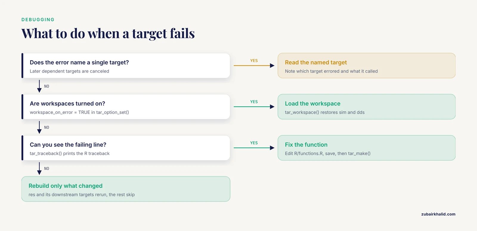
Break something on purpose to learn the loop. Inside extract_results(), change results() to resultss(), then run tar_make():
▶ dispatched target res
✖ error target res [0.01 seconds]
✖ canceled target report
R exits with an error naming res. Now turn on workspaces in _targets.R by adding workspace_on_error = TRUE inside tar_option_set(), rerun, and debug:
tar_workspace("res")   # loads dependencies and the failed target's context
tar_traceback("res")   # prints the R traceback for the failed command
tar_workspace() reconstructs the failed target's runtime environment in your interactive session, with sim and dds loaded and ready, so you can execute the failing command line by line exactly as targets ran it. Fix the function, save, and tar_make() rebuilds only res and its downstream targets.
Two more tools round out the toolkit. Setting error = "continue" on fragile, independent targets, or passing it to tar_make(), lets the rest of the pipeline finish while one branch fails, which is ideal for long per-sample steps. And tar_meta(fields = c("name", "warnings", "error")) surfaces silent warnings that did not stop the run.
Checking that the results are right
Automation removes transcription errors, not analysis errors. Build three habits into every pipeline. First, assert expectations inside targets, for example stop if colSums() on the count matrix returns zeros for any sample, so bad input fails loudly at the boundary. Second, read tar_meta() warnings after every run. Third, benchmark an automated pipeline against an established reference before trusting it. When a semi-automated homologous recombination deficiency workflow was compared with two commercial assays, genomic instability metrics correlated strongly across methods, with R-squared values up to 0.96, yet discordances concentrated in borderline cases near classification thresholds [12]. The lesson generalizes: agreement will look excellent overall and fail exactly where your decisions matter, so inspect borderline calls by hand.
Where to take the pipeline next
A few upgrades repay the effort once the demo works. Pin package versions with renv so the environment itself is reproducible, and add a container when you need portability beyond one machine. Move helper functions into packages once they stabilize. Split coarse targets at natural boundaries, one target per artifact you would hate to recompute, because finer granularity makes skipping sharper. Practical tips worth adopting early include naming targets after their outputs rather than their algorithms, keeping heavy I/O in dedicated targets with format = "file", and reviewing the graph with tar_visnetwork() after every structural change rather than after every failure.
Common Mistakes and Limitations
These are the errors that account for most lost hours with targets.
| Message or symptom | Cause | Fix |
|---|---|---|
| , - | , - | , - |
| Error in library(DESeq2) : there is no package called 'DESeq2' | Package missing on this machine, or not declared | Install it, then list it in tar_option_set(packages = ) |
| Error: object 'sim' not found | Typo in a dependency name inside a command | Match the tar_target() name exactly, then tar_make() |
| cannot open file '_targets.R': No such file or directory | tar_make() launched outside the project folder | Change into the project root, or set the TAR_PROJECT environment variable |
| A target reruns every time although nothing changed | External file tracked without format = "file", or a leftover cue with mode = "always" | Add format = "file" or restore the default cue |
| Branches rejected as incompatible | iteration = "vector" expects same-type branch values | Set iteration = "list" on the dynamic target |
Beyond the table:
- Editing objects in the console instead of functions. Fixes applied interactively are invisible to the graph, so the next tar_make() happily rebuilds stale outputs. Every fix belongs in R/functions.R.
- Calling set.seed() inside targets. It fights the per-target seeds targets already assigns. Delete it and rely on tar_option_set(seed = ) for reproducibility.
- Writing one giant target. A single target that reads, cleans, models, and plots can never be partially skipped. Split at each artifact boundary.
- Keeping everything in memory. Large pipelines exhaust RAM because finished outputs linger. Set memory = "transient" and garbage_collection = TRUE on heavy targets.
- Committing _targets/ to git or treating it as a backup. The store is a rebuildable cache. Ignore it in git and export final results to a durable folder you do track.
- Deleting _targets/ to force reruns. That discards every cached result. Use tar_force() from tarchetypes for one target, or a cue with mode = "always".
- Ignoring warnings in tar_meta(). A green pipeline with warnings is a pipeline with a hidden future failure.
Honest limitations. targets is R-first, so pipelines dominated by non-R command-line steps are expressible but require wrappers, and engines built for that world may fit better. targets also does not manage software installation, so pair it with renv, conda environments, or containers, and consider the packaging pattern of fully containerized, modular diagnostic frameworks with R front ends when work moves toward clinical use [13]. For multi-team production systems, the broader literature is clear that scripting alone does not provide the modularity, reusability, and maintainability that dedicated workflow systems contribute [4], so document why you chose targets and revisit the choice if the pipeline outgrows it.
Frequently Asked Questions
Is targets better than Snakemake or Nextflow for bioinformatics?
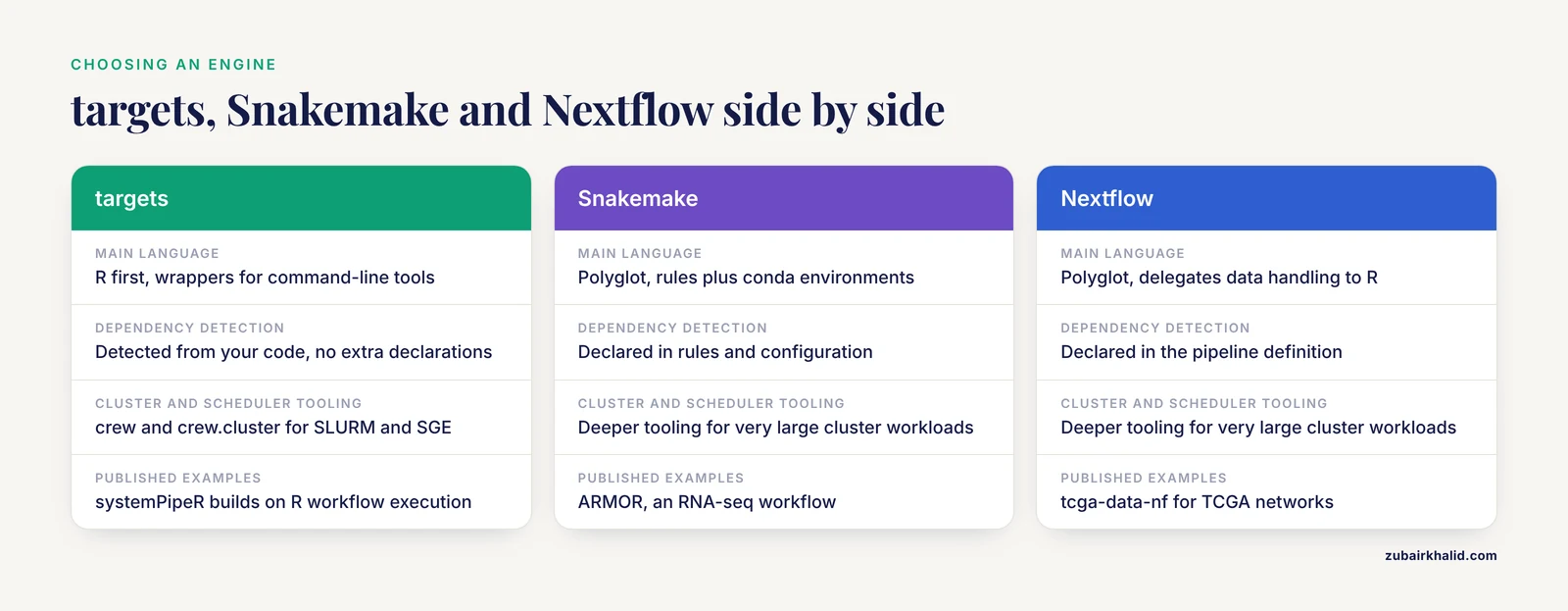
Neither wins everywhere. targets is the smoothest choice when the analysis lives in R, because dependencies are detected from your code without extra declarations. Snakemake and Nextflow have deeper tooling for polyglot pipelines and very large cluster workloads, which is why prominent published workflows such as ARMOR and tcga-data-nf were built on them.
How does targets decide which steps to rerun?
It hashes each target's command, function definitions, upstream data, package versions, and random seed, then compares against stored metadata. Anything that changed marks that target and everything downstream as outdated, and everything else is skipped.
Can targets run command-line tools such as FastQC or Trim Galore?
Yes. Call the tool with system2() inside a target, return the output path, and declare the target with format = "file" so targets tracks the produced files by content rather than by path alone.
How do I run a targets pipeline on an HPC cluster?
Use crew for parallel workers and crew.cluster for scheduler submission. crew.cluster provides controllers for common schedulers including SLURM and SGE, and you attach the controller once with tar_option_set(controller = ).
Where does targets store results, and should I commit them to git?
Results and metadata live in the _targets/ data store, which is a rebuildable cache. Add _targets/ to .gitignore, keep code under version control, and export final tables and reports to a durable results folder you do track.
How do I force one stubborn target to rerun?
Wrap it with tarchetypes::tar_force() or give it a cue with tar_cue(mode = "always"). Deleting the whole _targets/ folder also works but discards every cached result, so treat that as a last resort.
Does targets work with Bioconductor packages?
Yes. Install them with BiocManager and list them in tar_option_set(packages = ). targets records those packages as dependencies, so upgrading one reruns the targets that use it and skips the rest.
How is targets different from plain R scripts with saveRDS?
Scripts recompute everything and rely on you to remember what changed. targets derives the dependency graph from your code, skips up-to-date work, records provenance automatically, parallelizes independent steps safely, and gives every target a deterministic random seed.
Sources
- Developing reproducible bioinformatics analysis workflows for heterogeneous computing environments to support African genomics.
- An evolving computational platform for biological mass spectrometry: workflows, statistics and data mining with MASSyPup64.
- PyAutoFEP: An Automated Free Energy Perturbation Workflow for GROMACS Integrating Enhanced Sampling Methods.
- Developing and reusing bioinformatics data analysis pipelines using scientific workflow systems.
- systemPipeR: NGS workflow and report generation environment.
- ARMOR: An Automated Reproducible MOdular Workflow for Preprocessing and Differential Analysis of RNA-seq Data.
- Reproducible processing of TCGA regulatory networks.
- GCAC: galaxy workflow system for predictive model building for virtual screening.
- MeTime: an R package for reproducible longitudinal metabolomics data analysis.
- A Guide to Enzymatic Targeted Methylation Sequencing Bioinformatics Workflow: Best Practices.
- Genomic variant annotation workflow for clinical applications.
- Performance Assessment of a Locally Semi-Automated NGS-Based Workflow for Homologous Recombination Deficiency Testing in High-Grade Serous Ovarian Carcinoma.
- paRDal: bioinformatics framework for a parallel RNA and DNA NGS analysis in hereditary cancer diagnostics.