How to Create a Synteny Plot in R

By Dr. Zubair Khalid, DVM, MS, PhD · 2026-11-11

By the end of this guide you will be able to take two or more genome sequences, generate a pairwise alignment table with BLAST or MUMmer, and turn that table into a clean, publication-quality synteny plot in R, either as a dot plot or as a gene-order block map. You will also know which parameters control what you see, which errors to expect, and how to check that the plot is telling the truth about your genomes.

You need R 4.x installed, the packages ggplot2 and genoPlotR from CRAN, and optionally GenomicRanges and rtracklayer from Bioconductor. On the command line you need BLAST+ or MUMmer 4. Everything below runs on macOS and Linux and on Windows through WSL or RStudio's terminal.

What a Synteny Plot Shows

Synteny means conserved gene order across two or more genomes. Two regions are syntenic when the same genes, or the same sequence segments, occur in the same order and orientation, allowing for rearrangements such as inversions, translocations, duplications, and losses. A synteny plot is the visual summary of that comparison. It answers a simple biological question with a picture: which parts of genome A correspond to which parts of genome B, and how have they been rearranged?

The term appears constantly in comparative genomics papers because it carries real information. Synteny analyses have been used to confirm close relationships and reveal structural divergence in plant mitochondrial genomes [1], to support genus-level demarcation in Iridoviridae viruses alongside codon usage and phylogeny [2], and to show conserved mitogenome architectures across nematode superfamily Strongyloidea [3]. In chloroplast genomics, comparisons of Rosaceae plastomes are built on the observation that rose chloroplast genomes are generally conserved, with most species sharing identical inverted repeat boundaries [4]. Comparative synteny has even been used to infer the ancestry and fate of MIR160 homologs across Brassicaceae polyploids [5].

Dot Plots Versus Block Maps

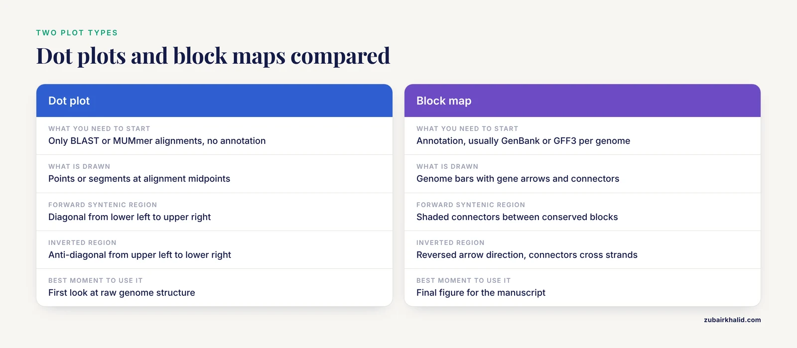
There are two main plot types, and you should choose deliberately between them.

A dot plot places one genome on the x axis and the other on the y axis. Every alignment hit between the two genomes becomes a point or a short segment at the intersection of its coordinates. A forward-syntenic region forms a diagonal line running from lower left to upper right. An inverted region forms an anti-diagonal running from upper left to lower right. Gaps in the diagonal are insertions or losses. Dot plots are the raw, unfiltered view, and they work without gene annotation. Dot plot analysis was used to explore genome synteny across 142 Salmonella prophage genomes alongside NUCmer alignments [6], and in classic human-mouse comparative sequencing work, dot plot analysis revealed surprisingly well-conserved sequence similarity across an entire orthologous region of human chromosome 11p15.3 and mouse chromosome 7 [7][8].

A block map (also called a gene-order or pangenome-style plot) draws each genome as a horizontal bar, genes as arrows or blocks along that bar in their annotated order, and colored connecting lines between homologous blocks. This is the style most readers recognize from chloroplast and mitochondrial genome papers. It requires annotation, usually a GenBank or GFF3 file per genome. Tools in this space include the Plant Orthology Browser, which pairs a gene-order visualization module with interactive dot plot representations of orthologous genes between chromosome pairs [9], and synphage, which generates synteny diagrams from GenBank files with genes color-coded by their degree of conservation across the displayed sequences [10].

A practical rule: start with a dot plot to see the raw structure, then build a block map for the figure that goes into the manuscript.

Choosing Your Toolchain in R

R for bioinformatics gives you three realistic routes to a synteny plot.

1. Direct plotting with ggplot2. You read an alignment table (BLAST tabular output or MUMmer coordinates) and draw it yourself. Full control, no black boxes, and the code doubles as documentation of your filtering decisions.
2. genoPlotR, a dedicated R package for plotting gene maps and comparisons between them, built around dna_seg and comparison objects.
3. Specialist upstream tools with R-friendly output. SyMAP computes raw hits with MUMmer, then clusters and filters them into synteny blocks and displays high-level dot plots and detailed drill-downs [11]. QUOTA-ALIGN screens synteny blocks in pairwise genome comparisons using binary integer programming, which matters enormously when one or both genomes have undergone whole genome duplication and naive one-to-one matching fails [12]. SyntenyQC is a Python command-line pre-processing tool for synteny plot construction that handles genomic data collection, annotation, and dereplication [13]. These tools sit before the plot, and their output can be loaded into R for final rendering.

This guide walks the ggplot2 route in detail and then shows the genoPlotR route, because together they cover almost every figure a comparative genomics paper needs.

How to Create a Synteny Plot in R, Step by Step

Step 1: Gather and quality-check the sequences

Download your genomes in FASTA format and get annotation (GenBank or GFF3) if you plan a block map. Before plotting anything, look at your inputs critically. SyntenyQC exists specifically because synteny plots are only as good as the data feeding them, and it supports collection, annotation, and dereplication to facilitate and sometimes fundamentally enable informative plots [13]. In practice this means removing redundant strains, checking that assemblies are the expected size and topology, and confirming annotation quality. A chloroplast genome should be roughly 120 to 165 kb, for example, and the two published plastomes you may compare against span 157,133 bp in Rosa platyacantha [4] and 139,633 bp in the microalga Ankistrodesmus falcatus [14]. A 400 kb "chloroplast genome" is a red flag before any plotting begins.

Name your files descriptively:

ls -lh *.fa
# cp_reference.fa   157 kb
# cp_query.fa       140 kb

Step 2: Generate pairwise alignments

You have two standard options.

Option A, BLASTN. Fast, transparent, and the output format is entirely under your control.

makeblastdb -in cp_reference.fa -dbtype nucl -out cp_ref
blastn -query cp_query.fa -db cp_ref \
  -outfmt "6 qseqid sseqid qstart qend sstart send pident length bitscore evalue" \
  -evalue 1e-5 -num_threads 4 -out ref_q.tsv

The -outfmt 6 argument writes a tab-delimited table with the ten columns you named, in that order. Each row is one local alignment between the query and the reference.

Option B, MUMmer's nucmer. Better when genomes are large or divergent, because it anchors on unique matches. SyMAP, for example, uses MUMmer to compute the raw hits between two genomes before clustering and filtering them into synteny blocks [11], and the Salmonella prophage study used NUCmer to evaluate linkages and correlations based on nucleotide identity between genomes [6].

nucmer -p ref_q cp_reference.fa cp_query.fa
show-coords -r -T -l ref_q.delta > ref_q.coords

The -p flag sets the output prefix, -T requests tab-delimited output, -r sorts alignments by reference position, and -l includes alignment lengths. Column layouts differ slightly between MUMmer versions, so open the file and confirm the order before parsing.

For the rest of the walkthrough I use the BLAST table, because its columns are fixed by your own -outfmt choice.

Step 3: Load and clean the alignment table in R

library(ggplot2)

cols <- c("qseqid", "sseqid", "qstart", "qend",
          "sstart", "send", "pident", "length",
          "bitscore", "evalue")

aln <- read.delim("ref_q.tsv", header = FALSE, col.names = cols)

# Midpoints for the dot plot, and a strand sign for each hit
aln$qmid <- (aln$qstart + aln$qend) / 2
aln$smid <- (aln$sstart + aln$send) / 2
aln$dir  <- sign(aln$qend - aln$qstart) * sign(aln$send - aln$sstart)

nrow(aln)
# e.g. 412
head(aln[, c("qmid", "smid", "pident", "dir")])

Two details matter here. First, BLAST coordinates are 1-based and inclusive, which matches how you think about positions in a sequence, but BED files are 0-based and half-open. If you import annotation from BED with Bioconductor's rtracklayer, coordinates shift by one, and mixing the two systems is a classic source of off-by-one plots. Second, the dir column encodes relative orientation: +1 means the hit is in the same orientation on both genomes, -1 means an inversion. Both signs are information, never discard them.

If your annotation is in GFF3, load it with Bioconductor and keep only the feature types you care about:

BiocManager::install(c("GenomicRanges", "rtracklayer"))

library(rtracklayer)
gff <- import("cp_query.gff3", format = "gff3")
cds <- gff[gff$type == "CDS"]

This is the standard Bioconductor tutorial pattern for converting annotation files into GRanges objects that can be filtered, overlapped, and exported.

Step 4: Draw the dot plot with ggplot2

The simplest honest version plots every alignment hit at its midpoint pair:

p <- ggplot(aln, aes(x = smid, y = qmid,
                     color = pident, shape = factor(dir))) +
  geom_point(size = 1.3, alpha = 0.75) +
  scale_color_viridis_c(name = "Identity (%)",
                        direction = -1) +
  scale_shape_manual(values = c("1" = 16, "-1" = 6),
                     labels = c("1" = "Same strand", "-1" = "Inverted"),
                     name = "Orientation") +
  labs(x = "Reference position (bp)",
       y = "Query position (bp)",
       title = "cp_query vs cp_reference") +
  theme_classic(base_size = 12)

print(p)

Expected output: one or more diagonal runs of points rising left to right, any inverted regions appearing as anti-diagonals marked with triangles, and scattered off-diagonal points representing repeats or spurious hits. For two closely related chloroplast genomes you would expect a single near-continuous diagonal, broken only at the inverted repeat boundaries, which is exactly the kind of boundary variation reported between algal plastomes [14].

For long alignments, segments communicate length better than points:

p2 <- ggplot(aln, aes(x = sstart, xend = send,
                      y = qstart, yend = qend,
                      color = pident)) +
  geom_segment(linewidth = 0.4, alpha = 0.8) +
  scale_color_viridis_c(name = "Identity (%)", direction = -1) +
  labs(x = "Reference position (bp)",
       y = "Query position (bp)") +
  theme_classic(base_size = 12)

print(p2)

Each segment now draws the actual extent of an alignment, so a 10 kb match looks like a 10 kb line rather than one pixel.

Step 5: Build a block map with genoPlotR

For the annotated, gene-arrow style figure, genoPlotR reads your gene tables and the block correspondences between them. Prepare two small tables, one per genome, with columns giving gene name, start, end, and strand:

library(genoPlotR)

# ref_genes.tsv: name  start  end  strand  col
#     rbcL  1002  2201  +  grey30
#     psaB  5400  8100  -  grey30
#     ...

ref_seg <- dna_seg(read.table("ref_genes.tsv", header = TRUE,
                              stringsAsFactors = FALSE))
qry_seg <- dna_seg(read.table("qry_genes.tsv", header = TRUE,
                              stringsAsFactors = FALSE))

# blocks.tsv: x1  x2  (reference start/end, query start/end per block)
#   1002  2201
#   5400  8100
#   ...

cmp <- comparison(read.table("blocks.tsv", header = TRUE,
                             stringsAsFactors = FALSE))

plot_gene_map(dna_segs = list(ref_seg, qry_seg),
              comparisons = list(cmp),
              main = "Reference vs query synteny")

The comparison() object links coordinates on the first segment to coordinates on the second, and plot_gene_map() draws the two genome bars with arrows for genes and shaded connectors for conserved blocks. Genes can be colored by functional category, which is how most chloroplast and mitochondrial figures distinguish photosystem genes, ribosomal genes, and transfer RNAs. The package vignette covers the optional columns that control connector color and width, and it is the authoritative reference for the full argument list.

Where do blocks.tsv coordinates come from? Either cluster your BLAST hits manually, or run a dedicated block-finding tool. The principled option for genomes with duplications is quota-based screening, which formulates block selection as a binary integer programming problem that maximizes total block score while respecting each genome's duplication history [12]. For small organelle genomes, manual curation of a few dozen blocks is often faster and more defensible.

Step 6: Export the figure

ggsave("dotplot.png", p, width = 6, height = 6, dpi = 300)
ggsave("dotplot.pdf", p, width = 6, height = 6,
       useDingbats = FALSE)

For journals, export PDF or SVG at the final column width, typically 85 to 90 mm for single column, and set base_size in your theme so text scales correctly. Save the alignment table and the plotting script together. A synteny figure that cannot be regenerated from its inputs will not survive peer review.

Key Parameters at a Glance

Synteny Plot in R Tips

Color by identity, not by block, in the dot plot. Identity gradients expose degraded alignments that a binary "syntenic or not" color scheme hides. In the Salmonella prophage comparison, genome sizes ranged from 6.4 to 358.7 kb and GC content from 35.5 to 65.4 percent [6], and only a gradient view would show where similarity thins out along such a range.

Repeat-hit discipline. A single repeated element, for example a transposon family, can produce hundreds of near-identical hits that camouflage the true diagonal. Filter by hit length as well as identity, or collapse hits per repeat family before plotting. This problem is acute in plant mitochondrial genomes, where one Arabis mitogenome carried 21.83 kb of transposable element sequence and 44.03 kb of repetitive DNA [15].

Facet by chromosome instead of stacking. When comparing multi-chromosome genomes, use facet_grid(query_chr ~ reference_chr, scales = "free") so each chromosome pair gets its own panel. A single panel with all pairs overlaid is unreadable and biologically misleading, since inter-chromosomal hits and intra-chromosomal repeats look identical.

Match the plot to the evolutionary distance. For closely related species, nucleotide-level dot plots carry everything you need. Across larger distances, syntenic signal lives in gene order rather than raw sequence identity, which is why studies of Brassicaceae MIR160 homologs leaned on comparative synteny rather than sequence similarity alone [5], and why tools like SyMAP allow micro-rearrangements inside larger blocks during block formation [11].

Let the plot genus delimit for you, cautiously. Synteny plus codon usage evidence has been used to support genus demarcation in Iridoviridae [2], and synteny analyses have confirmed close species relationships in Rhododendron [1]. A synteny plot is strong supporting evidence for a relationship, and it should sit alongside phylogeny rather than replace it.

Check boundary behavior explicitly. In quadripartite chloroplast genomes, the inverted repeat and single copy boundaries move between species, and that movement shows up as characteristic breaks near the ends of the dot plot diagonal. Lineage-specific IR/SC boundary variation is a documented feature of Sphaeropleales plastomes [14], so treat end-of-diagonal discontinuities in organellar plots as biology first and artifacts second.

Common Mistakes and Limitations

Plotting raw hits and calling them synteny. Raw alignment output is not a synteny analysis. SyMAP deliberately filters and clusters raw MUMmer hits before running its synteny algorithm, which is designed to tolerate micro-rearrangements while forming larger blocks [11]. If you skip the clustering step, repetitive DNA and short spurious matches will draw a noisy cloud over the diagonal you actually care about.

Assuming one-to-one matching. In genomes with whole genome duplication, a region in one genome corresponds to multiple regions in the other. Naive filtering throws away real signal or invents false uniqueness. QUOTA-ALIGN was built precisely to relax one-to-one requirements into one-to-many or many-to-many matchings while using an integer programming objective to control which blocks survive [12]. If your lineage has paleopolyploidy, quota screening is not optional.

Ignoring strand. The single most common plotting error is dropping the sign of the hit orientation. Inversions then vanish into the same diagonal as co-oriented hits, and the reader loses the rearrangement story entirely. The dir column in Step 3 exists so that this cannot happen silently.

Mixing coordinate conventions. BLAST and GFF3 are 1-based inclusive, BED is 0-based half-open. If a block appears shifted by exactly one base pair relative to its genes, this is why.

Overreading what the plot can prove. Synteny conservation supports common ancestry of a region, but it does not by itself establish orthology of every gene within a block, resolve gene tree discordance, or date divergence. Mycobacteriophage comparison illustrates the floor of the method: within a highly similar cluster, six genomes shared more than 97.5 percent average nucleotide similarity, while between two clusters similarity was barely detectable by diagonal plot analysis [7]. When the signal is that weak, absence of visible synteny is a statement about sequence divergence, not necessarily about absence of relatedness.

Plotting too many genomes in one figure. Dot plots are pairwise. Block maps scale poorly beyond roughly ten to fifteen genomes, at which point gene color coding by conservation grade, as synphage implements, communicates more than individual connectors [10]. For dozens of genomes, aggregate statistics or a matrix of selected pairwise plots beat one overloaded figure.

Dereplication failures. Including multiple near-identical strains distorts what the plot appears to show about conservation, because redundant sequences dominate the picture. SyntenyQC's dereplication step exists for exactly this reason [13], and the same discipline applies if you are filtering inputs by hand.

Annotation quality debt. A block map is a picture of your annotation as much as of your genome. Misannotated start codons, missing pseudogenes, and inconsistent feature naming between the two genomes will all render as apparent rearrangements. Reannotation of core genes changed conclusions in Iridoviridae work, where 23 core genes were re-determined by re-annotation, core-pan analysis, and local BLASTN before downstream analysis [2]. Budget time for this before plotting.

A final scope limit. Synteny plots describe genome-level correspondence. They cannot tell you expression, function, or selective pressure on their own, and any evolutionary claim drawn from them needs phylogenetic and, where relevant, selection analyses alongside it, as the Strongyloidea mitogenomic study combined synteny with codon usage and selection modeling [3].

How to Check That the Plot Is Right

Validate in three directions.

1. Internal consistency. The number of blocks in blocks.tsv should match the number of connectors in the genoPlotR figure and the number of diagonal runs in the dot plot. If these disagree, a filtering step is silently dropping rows.
2. Spot-check coordinates. Pick three genes at random, find their coordinates in the annotation file, and confirm they land at the plotted positions. A two-minute check catches coordinate-convention bugs that would otherwise reach print.
3. External sanity. Compare your result against published comparisons of the same or closely related taxa. For organellar genomes, published figures exist for most major lineages, and conserved architecture across a clade, such as the conserved mitogenome architectures reported across Strongyloidea [3] or the confirmed close relationship of Rhododendron simsii var. putuoense to R. simsii [1], gives you an expectation to test against.

Where to Go Next

Once the basic pairwise plot works, the natural extensions are multiple-genome block maps colored by conservation grade [10], quota-screened block sets for polyploid lineages [12], and quantitative summaries of the plotted blocks such as block length distributions and nucleotide diversity per region, the latter being how adaptive hot spots were flagged in the Rosa plastome comparison [4]. Keep the entire pipeline scripted from FASTA to final figure. Every parameter you tuned, from the BLAST evalue to the identity color scale, is a decision a reviewer may ask about, and a single script that reproduces the plot is the difference between answering confidently and guessing.

Frequently Asked Questions

What is the difference between a synteny plot and a dot plot?

A dot plot is one common type of synteny plot, showing every pairwise alignment hit as a point or segment between two coordinate axes. "Synteny plot" also covers block maps, which draw genomes as bars with gene arrows and colored connectors between conserved blocks. Dot plots are raw and annotation-free, block maps are curated and annotation-dependent.

Which R packages do I need for a synteny plot?

For the workflow in this article you need ggplot2 from CRAN for dot plots, genoPlotR from CRAN for gene-order block maps, and optionally GenomicRanges and rtracklayer from Bioconductor for handling GFF3 annotation. Install them with install.packages() and BiocManager::install() respectively.

Can I make a synteny plot without gene annotation?

Yes. Dot plots require only sequence-to-sequence alignments from BLAST or MUMmer, which is why they are the standard first look for unannotated assemblies. Block maps require annotation because they display gene order and identity, so an unannotated genome needs to be predicted and labeled first, or compared at the nucleotide level only.

How do I show an inversion in a synteny plot?

Inversions appear automatically in a dot plot as anti-diagonal runs of points descending from upper left to lower right. Encode the relative orientation of each alignment hit as a sign, as in the dir column in Step 3, and map it to a distinct point shape or color. In block maps, inverted genes are drawn with reversed arrow direction and connectors cross between opposite strands.

How many genomes can one synteny plot show?

Dot plots are strictly pairwise, one panel per genome pair. Gene-order block maps can stack many genomes vertically, but readability degrades beyond roughly ten to fifteen. For larger comparisons, color genes by their degree of conservation across the whole set rather than drawing individual pairwise connectors, which is the approach synphage takes for phage genome sets.

Why does my synteny plot look like noise instead of a diagonal?

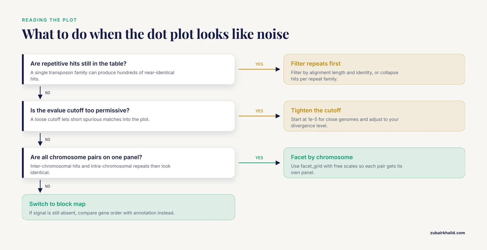
The usual causes are unfiltered repetitive hits, an evalue cutoff too permissive for your divergence level, plotting all chromosome pairs on one panel, or genuinely deep divergence where synteny lives in gene order rather than nucleotide sequence. Filter by alignment length and identity, collapse repeat families, facet by chromosome, and if signal is still absent, switch to an annotation-based block comparison.

How do I export a publication-quality synteny figure from R?

Use ggsave() with PDF or SVG output at the final journal column width, typically 85 to 90 mm for a single column, and set a base font size in your theme so all text scales together. genoPlotR plots can be saved through the standard graphics devices. Keep the script and the alignment table with the figure so the whole plot is reproducible.

Do synteny plots work for chloroplast and mitochondrial genomes?

Yes, and they are standard in that literature. Organellar genomes are small enough that a single pairwise dot plot plus one block map per figure covers the comparison, and conserved architecture across a clade gives a clear expectation. Published plastome comparisons in Rosa and Sphaeropleales and mitogenome comparisons in Rhododendron and Strongyloidea all use exactly this pairwise synteny framework.

Sources

1. Characterization of the complete mitochondrial genome of Rhododendron simsii var. putuoense and its comparative evolutionary analysis.
2. The Insights of Genomic Synteny and Codon Usage Preference on Genera Demarcation of Iridoviridae Family.
3. Comparative mitogenomics reveals evolutionary drivers of Strongyloidea nematodes dwelling in gastrointestinal tract.
4. Characteristics, comparative genomics, and phylogenetic analysis of the chloroplast genome of Rosaplatyacantha.
5. A prescient evolutionary model for genesis, duplication and differentiation of MIR160 homologs in Brassicaceae.
6. Comparative genomic analysis of 142 bacteriophages infecting Salmonella enterica subsp. enterica.
7. Comparative genomic analysis of 60 Mycobacteriophage genomes: genome clustering, gene acquisition, and gene size.
8. Comparative genomic sequencing reveals a strikingly similar architecture of a conserved syntenic region on human chromosome 11p15.3 (including gene ST5) and mouse chromosome 7.
9. The Plant Orthology Browser: An Orthology and Gene-Order Visualizer for Plant Comparative Genomics.
10. synphage: a pipeline for phage genome synteny graphics focused on gene conservation.
11. SyMAP v3.4: a turnkey synteny system with application to plant genomes.
12. Screening synteny blocks in pairwise genome comparisons through integer programming.
13. Synteny plot quality control with SyntenyQC.
14. Decoding the first complete chloroplast genome of the Amazonian oleaginous microalga Ankistrodesmus falcatus: architecture, codon usage, and comparative genomics within the Sphaeropleales.
15. Mitochondrial Genome of the Korean Endemic Arabis takesimana (Brassicaceae): Addition to the Genomic Resources and Evolutionary Insights.