How to Quantify Gene Expression with StringTie

By Dr. Zubair Khalid, DVM, MS, PhD · 2026-11-11

By the end of this guide you will be able to take a folder of RNA-seq FASTQ files, align them, assemble transcripts, merge assemblies across samples, and produce a clean matrix of gene and transcript counts plus TPM values that feeds directly into differential expression tools such as DESeq2 or edgeR. Everything runs on a standard Linux or macOS workstation with at least 16 GB of RAM, and every command shown here can be copied and adapted to your own data.

This StringTie tutorial walks through gene expression quantification step by step, explains each parameter that actually changes your results, shows the errors you will hit and how to fix them, and covers how to verify that your numbers are real before you publish or build on them. If you want to learn bioinformatics from the analysis side rather than the theory side, quantification is one of the best skills to practice because the output is concrete and easy to sanity check.

What StringTie Does and Where It Fits in a Pipeline

StringTie is a transcript assembly and quantification program developed at the Center for Computational Biology at Johns Hopkins, the same group behind HISAT2 and Ballgown. It takes splice-aware alignments in BAM format and does two jobs:

1. Assembly. It reconstructs transcript structures from the read alignments, including isoforms and novel transcripts that are not in your reference annotation.
2. Quantification. It estimates expression for every transcript and gene it knows about, reporting coverage, FPKM, and TPM.

TPM stands for transcripts per million. It normalizes expression first by transcript length and then by the total pool of transcripts in the sample, so TPM values sum to one million within each sample and are comparable across samples. FPKM, fragments per kilobase of transcript per million mapped reads, normalizes in the opposite order, which makes cross-sample comparison less reliable. This distinction matters when you choose which column to use downstream.

StringTie does not do differential expression. Its job ends at producing accurate expression values. Everything after, such as the differential expression calls, enrichment analysis, and network construction seen in published RNA-seq studies, happens in R or Python. For example, a recent tea flower study quantified mRNA and small RNA expression across seven dissected floral tissues from 21 samples and went on to identify 33,333 nonredundant differentially expressed genes across tissue comparisons [1]. A wheat study used strand-specific RNA-seq to identify 2,736 expressed long intergenic noncoding RNAs during stripe rust infection, of which 515 were differentially expressed [2]. Both analyses sit downstream of exactly the kind of quantification step this guide teaches.

Prerequisites

Install these before starting. The fastest route is Conda, which resolves dependencies for you.

conda create -n rnaquant -c bioconda -c conda-forge \
  stringtie hisat2 samtools gffcompare prepde \
  python=3.10
conda activate rnaquant

Check that everything works:

stringtie --version
hisat2 --version | head -1
samtools --version | head -1
gffcompare --version

Expected output looks like this (your versions may differ):

2.2.1
2.2.1
1.17
gffcompare v0.12.6

You also need on hand:

• Raw RNA-seq reads in FASTQ format, ideally gzip compressed.
• A reference genome FASTA and a matching GTF annotation file from the same genome build. For human work, use the GENCODE release or the Ensembl release corresponding to GRCh38. For mouse, use GRCm39. The critical rule is that your genome FASTA, GTF, and alignment index all come from the same build.
• Sample metadata, including strandedness of the library, which is one of the most common silent sources of error covered later.

If you prefer to build StringTie from source rather than use Conda, download the tarball from the official StringTie page at the Johns Hopkins Center for Computational Biology website and run make release. The binary appears in the top level of the source directory. Conda is simpler and reproducible, so use it unless you have a reason not to.

Step by Step: Quantifying Expression with StringTie

This walkthrough uses three example samples, control_rep1, treated_rep1, and treated_rep2, mapped against human GRCh38. Replace paths and sample names with your own. The same workflow works for any organism with a genome assembly and GTF.

Step 1. Build the alignment index and confirm your annotation

# Download Ensembl GRCh38 genome and GTF (adjust release number)
wget https://ftp.ensembl.org/pub/release-109/fasta/homo_sapiens/dna/Homo_sapiens.GRCh38.dna.primary_assembly.fa.gz
wget https://ftp.ensembl.org/pub/release-109/gtf/homo_sapiens/Homo_sapiens.GRCh38.109.gtf.gz
gunzip *.gz

# Build HISAT2 index (splicesites extracted from GTF improve alignment)
hisat2_extract_splice_sites.py Homo_sapiens.GRCh38.109.gtf > splice_sites.txt
hisat2-build -p 8 Homo_sapiens.GRCh38.dna.primary_assembly.fa GRCh38_index

Before going further, check one chromosome naming question: does your GTF use chr1 or 1? Ensembl uses 1. UCSC uses chr1. StringTie will not error out loudly when these mismatch. It will quietly assign expression to nothing, and you will discover the problem only when every TPM in your output is zero. Look at the first line of your GTF:

head -2 Homo_sapiens.GRCh38.109.gtf

If the GTF says 1 and your alignments will say chr1, fix it now with a one line rename or download annotations from a source whose naming matches your genome FASTA.

Step 2. Align reads with HISAT2 using the dta flag

hisat2 -p 8 --dta \
  -x GRCh38_index \
  -1 control_rep1_R1.fq.gz -2 control_rep1_R2.fq.gz \
  | samtools sort -@ 4 -o control_rep1.bam
samtools index control_rep1.bam

The -dta flag tells HISAT2 to report alignments in a format optimized for downstream transcript assembly by StringTie. It changes how HISAT2 handles reads that span exon junctions. If you omit it, alignment succeeds and StringTie runs, but assembly quality degrades in ways that are hard to see without careful checking. This omission is one of the most common mistakes in this pipeline and it produces no error message.

Check the alignment summary:

hisat2 -p 8 --dta -x GRCh38_index \
  -1 control_rep1_R1.fq.gz -2 control_rep1_R2.fq.gz \
  -S /dev/null 2> align_summary.txt
cat align_summary.txt

Typical output for a decent mammalian RNA-seq library:

1000000 reads; of these:
  1000000 (100.00%) were paired; of these:
    893421 (89.34%) paired aligning uniquely
    45110 (4.51%) aligned concordantly multiple times
    ...
overall alignment rate 95.11%

For well prepared mammalian libraries you generally expect overall alignment rates well above 80 percent. A rate in the 40 to 60 percent range usually means contamination, wrong reference species, or heavily degraded RNA. Stop and investigate before quantifying, because StringTie cannot rescue bad alignments. Repeat the alignment and indexing commands for every sample. A simple loop handles it:

for sample in control_rep1 treated_rep1 treated_rep2; do
  hisat2 -p 8 --dta -x GRCh38_index \
    -1 ${sample}_R1.fq.gz -2 ${sample}_R2.fq.gz \
    | samtools sort -@ 4 -o ${sample}.bam
  samtools index ${sample}.bam
done

Step 3. Assemble transcripts for each sample against the reference

stringtie control_rep1.bam \
  -G Homo_sapiens.GRCh38.109.gtf \
  -o assembly/control_rep1.gtf \
  -A abundance/control_rep1.tsv \
  -p 8

Here is what each option does:

At this stage you have not quantified against a common transcript set yet. You have one assembly per sample, which is the correct intermediate result.

Step 4. Merge assemblies into a unified transcript set

Different samples reveal different transcripts. To compare samples fairly you need one catalog of transcripts used for every sample. StringTie provides a merge mode for this:

ls assembly/*.gtf > gtf_list.txt
stringtie --merge -G Homo_sapiens.GRCh38.109.gtf \
  -o merged.gtf -p 8 gtf_list.txt

The merged GTF contains all reference transcripts plus any novel isoforms or intergenic transcripts that StringTie found reliably across samples. Novel assembled transcripts receive placeholder identifiers of the form MSTRG.123 followed by MSTRG.123.1, MSTRG.123.2 for isoforms. Seeing MSTRG prefixes in your output is normal and expected. It simply means the transcript came from assembly rather than the reference annotation.

Optionally compare the merged assembly to the reference to classify novelty:

gffcompare -r Homo_sapiens.GRCh38.109.gtf -o gffcmp merged.gtf
cat gffcmp.stats

The stats file summarizes class codes. Transcripts marked with = match the reference exactly, j are novel isoforms of known genes, u are intergenic novel transcripts, and o overlap reference transcripts in complicated ways. If your u count is enormous relative to your reference gene count, double check that the right GTF and genome build were used, because misbuilt assemblies frequently generate spurious intergenic transcripts.

Step 5. Run the final quantification pass with -e

Now rerun StringTie on each BAM, but this time with the merged GTF and estimation restricted to known transcripts:

for sample in control_rep1 treated_rep1 treated_rep2; do
  stringtie ${sample}.bam \
    -e -B -G merged.gtf \
    -o ballgown/${sample}/${sample}.gtf \
    -A abundance_final/${sample}.tsv \
    -p 8
done

The -e flag tells StringTie to skip assembly and only estimate expression for transcripts in the merged GTF. This is the pass that produces the numbers you will actually analyze. The -B flag writes Ballgown table files, including ctab files per sample, which is optional but convenient if you plan to use Ballgown in R.

One conceptual point that confuses many newcomers: the assembly pass in Step 3 and the quantification pass in Step 5 use the same command structure but produce different outputs because of the flags. The assembly pass finds transcripts. The quantification pass measures them consistently across all samples.

Step 6. Build gene and transcript count matrices with prepDE

StringTie writes one abundance file per sample. Differential expression tools need a single matrix with samples as columns. The StringTie package includes prepDE.py3 for exactly this:

# Create a sample list file mapping sample names to their GTF paths
cat > sample_list.txt <<EOF
control_rep1 ballgown/control_rep1/control_rep1.gtf
treated_rep1 ballgown/treated_rep1/treated_rep1.gtf
treated_rep2 ballgown/treated_rep2/treated_rep2.gtf
EOF

prepDE.py3 -i sample_list.txt \
  -g gene_counts.csv \
  -t transcript_counts.csv \
  -l 100

The -l flag sets the mean read length used when estimating counts from coverage, which for most modern Illumina libraries is around 100 to 150 bp. Check your actual read length with head -1 control_rep1_R1.fq.gz | wc -c and subtract one for the newline.

The output files look like this:

gene_id,control_rep1,treated_rep1,treated_rep2
ENSG00000223972,0,0,0
ENSG00000227232,48,51,39
ENSG00000243485,912,1043,867
ENSG00000288555,214,198,233

gene_counts.csv holds estimated raw counts suitable for DESeq2 and edgeR. transcript_counts.csv holds the same at transcript resolution.

Step 7. Understand the abundance table columns

Open one final-pass abundance table:

column -t abundance_final/control_rep1.tsv | head -6

Gene ID      Gene Name  Reference  Strand  Start      End        Coverage  FPKM   TPM
ENSG0000018  ALK        ENSG00000  +       29192773   29317945   4.115     8.231  9.847
ENSG0000001  BACE1      ENSG00000  +       1166592    1173211    1.054     2.108  2.522

The columns follow the StringTie specification directly. Coverage is average per-base read depth across the gene. FPKM scales coverage by transcript length and library size. TPM rescales so that all TPM values in a sample sum to exactly one million.

You can verify the TPM property yourself in one line:

awk -F'\t' 'NR>1 {s+=$9} END {print s}' abundance_final/control_rep1.tsv

Expected output: 1000000, sometimes with a tiny floating point remainder such as 999999.98.

Step 8. A worked TPM calculation

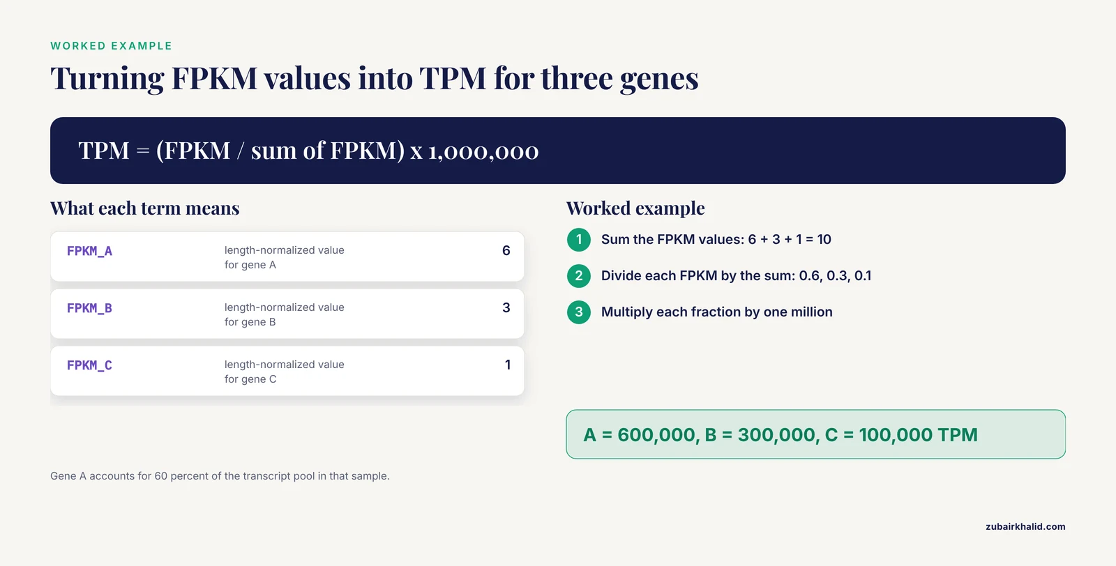
To see where TPM comes from, imagine a toy sample with mapped reads covering only three genes. After length normalization, suppose StringTie reports FPKM values of 6, 3, and 1 for genes A, B, and C.

1. Sum the FPKM values: 6 + 3 + 1 = 10.
2. Divide each FPKM by the sum: A = 0.6, B = 0.3, C = 0.1.
3. Multiply by one million: A = 600,000 TPM, B = 300,000 TPM, C = 100,000 TPM.

Gene A now accounts for 60 percent of the transcript pool in that sample. Because the denominator is the total transcript pool rather than the total mapped reads, TPM values remain comparable between samples with different sequencing depths, which is why TPM is the right choice for within-sample questions such as which gene dominates a tissue or which isoform dominates a locus.

For between-sample differential expression, however, use the raw estimated counts from prepDE.py3 with DESeq2 or edgeR. Those tools apply their own normalization and variance modeling. Feeding TPM values into DESeq2 is a well documented mistake because TPM discards the count information that the statistical model needs.

Where Quantification Ends and Analysis Begins

The count matrix is the handoff point between this tutorial and the rest of transcriptomics. Most published studies take expression matrices and perform differential expression, pathway enrichment, co-expression network analysis, and validation. Recognizing this pattern in the literature helps you understand why quantification quality matters so much upstream.

A chicken coccidiosis study combined transcriptome sequencing with immune measurements and challenge assays across infection time points, and found that the six day post infection stage represented the peak of the host immune response, driven by pathways including the NF-κB mediated coagulation and complement cascade [3]. A rice study integrated RNA-seq based co-expression network analysis with QTL mapping and qRT-PCR validation to prioritize the salinity tolerance candidate gene OsFBX29 [4]. A livestock study ran differential expression, WGCNA, and cis-eQTL mapping on blood transcriptomic data from lambs to dissect feed efficiency traits [5]. A study of mass reared versus wild fruit flies used PCA to separate transcriptomes by group, identified more than 1,300 differentially expressed genes per strain, and then ran GO and KEGG enrichment [6]. In each case, every downstream number depended on the expression estimates produced at the quantification step you just completed.

Novel transcripts from the merge step also matter in real studies. The wheat lincRNA work mentioned earlier identified its differentially expressed long intergenic RNAs from strand-specific RNA-seq data assembled against the genome, then linked them to defense pathways and built a competing endogenous RNA regulatory network around 65 of them [2]. StringTie assembly mode plus careful novelty classification is the standard route to that kind of finding in non-model organisms.

Common Errors, Their Exact Messages, and Fixes

These are the failures you are most likely to meet, in rough order of frequency.

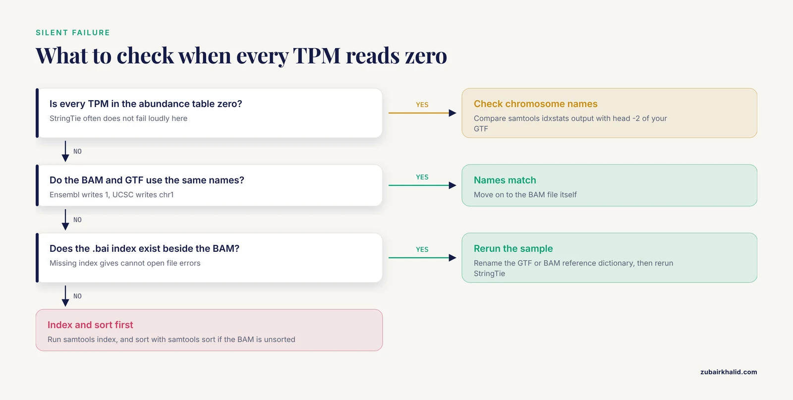
Every TPM in the output is zero. The cause is almost always a chromosome naming mismatch between the BAM and the GTF, for example Ensembl 1 versus UCSC chr1. StringTie will not always fail loudly. Run samtools idxstats control_rep1.bam | head and compare chromosome names to head -2 your.gtf. If they differ, rename either the GTF with awk or the BAM reference dictionary with samtools reheader, then rerun.

"Error: cannot open file" or similar when loading the BAM. The BAM index is missing or was not created. Run samtools index sample.bam and confirm the .bai file exists in the same directory.

The input alignment file is not sorted. StringTie requires position-sorted BAM. Pipe HISAT2 output through samtools sort as shown in Step 2. Sorting after the fact with samtools sort -o sorted.bam unsorted.bam also works, followed by indexing.

prepDE reports that transcript IDs do not match across samples. You built the matrices from per-sample GTFs produced in assembly mode instead of the final -e pass against a merged GTF, or you used the reference GTF in one sample and the merged GTF in another. Every sample in the matrix must be quantified against the identical merged GTF. Rerun Step 5 for all samples with the same -G merged.gtf.

All counts look unexpectedly low, roughly half or less of what similar published data show. The most likely cause is wrong strandedness. If your libraries are stranded and you ran StringTie without -rf or -fr, reads antisense to the transcript still contribute to coverage in the wrong direction and the estimator undercounts. Confirm library strandedness from the library preparation protocol, then rerun with the correct flag. As a diagnostic, rseQC infer_experiment.py reports the strandedness balance directly from the BAM.

Assembly produces thousands of tiny transcripts with poor support. You likely ran assembly on alignments made without HISAT2 -dta, or your coverage and isoform fraction thresholds are too permissive for your depth. Realign with -dta, and consider -c 2.5 -f 0.1 for high-depth libraries.

hisat2 reports very low alignment rates. Causes include the wrong species or genome build, adapter contamination, or severely degraded RNA. StringTie will run on whatever it receives, so this failure mode is silent downstream. The fix belongs upstream: verify the reference, run FastQC, and trim adapters if needed.

gffcompare complains about unknown chromosomes or produces mostly unknown class codes. Same root cause as the zero TPM problem, a build or naming mismatch. Align your chromosome vocabularies across FASTA, GTF, BAM, and merged GTF before comparing.

How to Check That Your Quantification Is Right

Verification separates a trustworthy matrix from garbage that will poison every downstream plot. Run these checks before differential expression.

Distribution sanity. Plot a density histogram of log2 TPM plus 1 per sample. Well behaved RNA-seq samples show a dominant peak around zero (most genes off) with a long right tail. A sample whose distribution is shifted relative to its group suggests a depth or quality problem.

TPM totals. As in Step 7, confirm each sample's TPM column sums to one million. Samples that do not sum correctly indicate a truncated file or an interrupted run.

Correlation and PCA. Compute pairwise Pearson correlations of log2 TPM across samples. Biological replicates within a condition should cluster tightly. Then run PCA on the top variable genes. A fruit fly transcriptomics study cited earlier used PCA precisely this way to separate mass-reared strains from wild individuals, with clean separation of groups on the first principal component [6]. If your treated and control replicates intermix on PC1 with condition, suspect batch effects or sample swaps.

Known marker check. Pick five genes you expect to be highly expressed in your tissue and five you expect to be silent, and look up their TPMs. Housekeeping genes such as ACTB, GAPDH, and RPLP0 should be present in the upper TPM range in most mammalian tissues. This five minute check catches annotation mismatches faster than any statistical test.

Cross-tool concordance. For one sample, quantify with StringTie and separately count reads with featureCounts or estimate with Salmon. Spearman correlation between the two gene-level TPM or count vectors should be high for well annotated genes. Large systematic disagreement on a subset of genes usually points to duplicated or paralogous loci, where multi-mapping reads are handled differently by each tool.

Novel transcript support. If you rely on MSTRG transcripts, check their coverage and the class codes from gffcompare. In organisms with complex or polyploid genomes, such as wheat, annotation incompleteness is common and assembly-based discovery is productive, but requiring solid coverage before trusting novel loci is standard practice, as the wheat lincRNA study illustrates with its filtered set of 515 differentially expressed candidates from 2,736 identified [2].

Common Mistakes and Limitations

These mistakes appear repeatedly in real projects, including projects by experienced analysts. Treat this as a preflight checklist.

Running -e during assembly and losing novel transcripts. The -e flag restricts output to reference transcripts. If you apply it in the first pass, StringTie never reports anything your GTF lacks, and you will never discover novel isoforms. Reserve -e for the final quantification pass only.

Quantifying each sample against a different transcript set. Every sample must be measured against the same merged GTF, built from all samples, before you make matrices. Mixing per-sample assemblies breaks identifier consistency and makes the count matrix meaningless.

Using TPM for differential expression. TPM answers within-sample questions. Differential expression answers between-sample questions and needs raw counts with DESeq2, edgeR, or an equivalent model. Both numbers come from the same StringTie run. Use each for its own purpose.

Ignoring strandedness. An unflagged stranded library silently halves or distorts expression estimates. Record library strandedness in your metadata sheet at the sequencing stage, not when you first see strange results six months later.

Mixing genome builds or annotation versions mid-pipeline. The FASTA, GTF, HISAT2 index, and merged GTF must all derive from one build. Annotation updates are welcome between projects, never within one.

Treating a merge of many shallow assemblies as truth. StringTie merge reduces noise by requiring support across samples, but very low depth samples contribute weak assemblies. If one sample contributes a suspicious fraction of novel transcripts, check its library size and alignment quality.

Forgetting batch structure. Quantification is per-sample and blind to experimental design. Batch effects live in the expression values themselves. Modern reanalysis projects handle this by reprocessing public data through a unified pipeline with standardized quality control and explicit batch-effect correction before cross-study integration [7]. Design your own experiment so that conditions are balanced across batches, and model batch terms in your differential expression analysis.

Expecting StringTie to solve scRNA-seq. StringTie is built for bulk and SMART-style full-length transcript work. Single-cell analyses use dedicated tools such as Cell Ranger, STARsolo, or alevin-fry, and their analysis frameworks, from clustering and trajectory inference to pseudobulk differential expression on cell-aggregated counts, differ substantially from bulk workflows [8]. Do not repurpose a bulk pipeline for droplet data without changing tools.

Over-trusting a single quantifier. Different estimators make different assumptions about multi-mapping reads and annotation completeness. For genes near the center of your biological claim, confirm expression with an orthogonal method. Published studies routinely validate key findings by qRT-PCR, as the rice salinity tolerance work did for its candidate gene [4].

Next Steps After Quantification

Once gene_counts.csv is in hand, the standard path is:

1. Import counts into R with DESeq2 or edgeR. Filter low-count genes, apply size-factor or TMM normalization, fit the model with your design formula, and extract differential expression results.
2. Annotate and visualize. MA plots, volcano plots, heatmaps of top variable genes, and PCA replicate the checks from the verification section at a more formal level.
3. Pathway and network analysis. Overrepresentation analysis with GO and KEGG, or WGCNA module construction, connects your gene lists to biology. The tea flower study built 24 co-expression modules from quantified tissue expression and linked three module eigengenes to specific floral traits [1].
4. Validate. qRT-PCR on a handful of top genes remains the standard confirmation step in the RNA-seq literature [4].

If your long-term goal includes building your own analysis skills rather than following recipes, the discipline of verifying each intermediate output, alignment rates, TPM sums, correlation structure, marker genes, is the habit that distinguishes reproducible work from fragile work. A structured bioinformatics course accelerates this, but the verification habit is learnable right here with your own data.

Frequently Asked Questions

Does StringTie output raw counts or TPM?

StringTie outputs coverage, FPKM, and TPM per transcript and gene in its abundance tables, and estimated raw counts are generated separately by the included prepDE.py3 script. Use counts with DESeq2 or edgeR and TPM for within-sample comparisons.

When do I use the -e and -B flags?

Use -e only in the final quantification pass against a merged GTF, when you want expression for known transcripts without assembly. Use -B in the same pass if you plan to analyze results with the Ballgown R package. Never use -e in the initial assembly pass or you will lose novel transcripts.

Do I need to run stringtie, merge?

Yes, if you have more than one sample and plan to compare them. The merge step creates one transcript catalog containing reference transcripts plus novel isoforms found across samples, and quantifying every sample against that single catalog is what makes the count matrix valid.

Can StringTie quantify expression without an annotation file?

Yes, StringTie can assemble and estimate expression in de novo mode when no GTF is provided, but gene and transcript names will all be MSTRG placeholders and interpretation requires mapping assembled transcripts to a reference afterward. For standard differential expression work, always provide a reference GTF.

What is the difference between TPM and FPKM?

Both normalize by transcript length and sequencing depth, but in opposite order. TPM normalizes by length first and then scales so TPM values sum to one million per sample, making TPM the preferred within-sample measure. FPKM divides by total mapped reads first, which makes FPKM values harder to compare across samples.

Why do my transcript IDs start with MSTRG?

MSTRG identifiers are assigned by StringTie to transcripts that came from its own assembly rather than the reference annotation. Novel isoforms appear as MSTRG.numeric.suffix and can be linked to nearby reference genes using the gffcompare class codes.

What aligner should I use before StringTie?

HISAT2 with the -dta flag is the pairing the StringTie developers designed and recommend. STAR is also widely used with StringTie by converting its output appropriately. The essential requirement is a splice-aware aligner, and for HISAT2 the -dta flag specifically improves downstream assembly.

Can I use StringTie for single-cell RNA-seq data?

No, not as the primary quantifier. Droplet-based single-cell libraries have 3-prime or tag-based structure and enormous cell numbers that bulk quantifiers do not handle, and single-cell analysis frameworks rely on cell-level count matrices from dedicated tools. StringTie remains an excellent choice for bulk RNA-seq and full-length transcript quantification.

Sources

1. Integrated RNA-seq and small RNA-seq profiling reveals tissue-associated transcriptional programs and candidate miRNA-mRNA relationships across tea floral tissues.
2. Identification and expression analysis of intergenic long non-coding RNAs (lincRNA) associated with stripe rust resistance in wheat.
3. Transcriptomic analysis of cecal mucosal immunity in SPF White Leghorn chicks infected with precocious and parent strains of Eimeria tenella.
4. QTL mapping and haplotype analysis reveal candidate genes for seedling-stage salinity tolerance in rice.
5. Genome-wide cis-expression Quantitative Trait Loci (eQTL) and transcriptomic signals reveal distinct molecular regulation across correlated feed efficiency traits.
6. Comparative transcriptomic analysis of functional and metabolic changes in mass-reared and wild Anastrepha ludens Loew (Diptera: Tephritidae).
7. Integrative transcriptomics and hypothesis-driven transfer machine learning reveal conserved and species-specific host-parasite dynamics across Leishmania species in THP-1 cells: a systematic review and meta-analysis.
8. Using In Silico Pseudobulk Differential Expression and Trajectory Analysis of Single Cell RNA Sequencing to Reveal Stem Cell State Transitions in Colonic Inflammation.