How to Start a Bioinformatics Study Group
By Dr. Zubair Khalid, DVM, MS, PhD ·

By the end of this guide you will have a written charter, a shared code repository with a pinned software environment, a six-week session plan, and a meeting format that survives busy weeks. You will also have run a small quality-control analysis on sequencing data together, on every member's laptop, with identical results on every machine.
You need four things on hand before you start:
- A laptop where you can install software (administrator rights)
- About two hours per week, one for the meeting and one for homework
- A free account on a git hosting service such as GitHub, plus git installed locally
- Three to seven colleagues, classmates, or friends who also want to learn bioinformatics
A formal bioinformatics course supplies a syllabus, lectures, and deadlines. A study group supplies accountability, live debugging, and the social pressure that keeps people going after week three. The two combine well. This guide builds the group half of that pairing: recruiting, format, infrastructure, curriculum, and the habits that carry a group past its first season.
Why a study group is the right vehicle for learning bioinformatics
Bioinformatics is wider than any one person's job. During the first months of the COVID-19 pandemic, research groups around the world redirected effort into computational work, and a bibliometric review of 184 articles found that metagenomics and transcriptomics were the main data sources, with phylogenetic analysis used to confirm zoonotic transmission and protein sequence analysis, immunoinformatics, and molecular docking used to probe drug and vaccine targets [1]. If entire laboratories narrowed themselves to a small method set in order to move fast, a study group with two hours a week certainly must.
Most newcomers also arrive from the wet lab or the clinic, not from computer science. A practical guide written for medical researchers without a bioinformatics background walks through study design, sample collection, the role of negative and positive controls, multiple-comparison problems, and step-by-step analysis pipelines [2]. That is exactly the kind of material a group can digest together, because someone catches your typos and someone explains the statistics you were too embarrassed to ask about alone.
The third reason is that the field's core skill is reproducibility, and reproducibility is a team sport. An environment file that works on one laptop means nothing until four other people have run it. A study group forces that confrontation early, on a toy dataset, instead of late, on a grant deadline.
How to Start a Bioinformatics Study Group in Seven Steps
The steps below take roughly three weeks from first conversation to first session. Steps 1 through 3 are decisions, Step 4 is an evening of setup, Steps 5 through 7 are the running rhythm.
Step 1: Choose one narrow track before you recruit anyone
"Learn bioinformatics" is not a goal. Pick a track that ends in a concrete artifact, because the artifact is what you advertise when you recruit and what you grade yourselves against in week twelve. The five tracks below cover most first groups, and each maps onto work that the field actually publishes.
| Track | Core question you can answer | Representative tools | First-semester milestone |
|---|---|---|---|
| RNA-seq differential expression | Which genes change between two conditions? | FastQC, MultiQC, an aligner or pseudoaligner, DESeq2 in R | A volcano plot built from a public count table |
| Microbiome and metagenomics | Which organisms are present, and which groups differ? | Amplicon pipelines plus R for diversity statistics [2] | Alpha and beta diversity figures from a public dataset |
| Comparative genomics | How do related microbial genomes differ? | Web platforms such as EDGAR for ortholog group analysis [3] | An ortholog table and a phylogenetic tree for ten genomes |
| Cancer prognosis screening | Which genes associate with survival? | Survival web servers such as KM plotter [4] | One Kaplan-Meier curve with a written caveat list |
| Sequence-based protein analysis | What do sequence features suggest about a protein family? | UniProt entries, charge and disorder profiles [5] | A short written report on one protein family |
A few terms in that table deserve definitions. Orthologs are genes in different species that descend from a common ancestral gene. Beta diversity is the difference in community composition between samples, as opposed to alpha diversity, which is diversity within one sample. Amplicon data comes from sequencing a specific marker gene, most commonly the 16S ribosomal RNA gene for bacteria.
Resist the temptation to copy the most impressive papers in your field. Integrative oncology studies routinely chain differential expression analysis, weighted gene coexpression network analysis (WGCNA, a method that groups genes into modules based on correlated expression across samples), protein-protein interaction network analysis to find hub genes, and molecular docking (computational prediction of how a small molecule binds a protein) [6]. That chain is a full semester of work, not a first session. Start smaller than the papers you admire, then grow toward them.
Step 2: Recruit four to eight people and set expectations
Four to eight members is the practical sweet spot. Below four, one dropout halves the group and the presenter rotation collapses. Above eight, the troubleshooting circle turns into an audience. Three is enough to begin, and groups can grow later.
Look sideways before you look up. Lab mates, fellow graduate students, clinicians on your service, analysts at the local public health department, and classmates from a statistics course are all better recruits than a professor you hope will lecture at you. Post a short message on department listservs, in lab meeting announcements, or in online communities that have a local channel. A workable invitation looks like this:
Subject: Bioinformatics study group, 90 minutes per week

I am starting a 12-week study group on RNA-seq data analysis.
We meet Tuesdays 16:00-17:30, hybrid (room 2.14 plus a video call).
Each week one member drives a hands-on session and everyone types along.
Homework takes under two hours. First meeting: March 4.
Reply if you want in, we cap at eight people.
Set three expectations in the first reply to every interested person. First, attendance: the charter below suggests eight of twelve sessions. Second, equipment: a laptop they can install software on, not a tablet. Third, homework: under two hours per week, always producing a file that goes into the shared repository. People accept honest constraints. They quit over vague ones.
Step 3: Pick a format and write the rules down
The format is the answer to one question: what happens during the ninety minutes? Different mixes of people need different answers.
| Format | Best for | Cadence | First artifact |
|---|---|---|---|
| Paper-to-pipeline club | Members who want to read and reproduce literature | Biweekly, 90 minutes | One reproduced figure |
| Tool deep dive | Clinicians who need quick, practical answers | Weekly, 60 minutes | A written cheat sheet per tool |
| Course cohort | Beginners who want the structure of a bioinformatics course | Weekly, 90 minutes | Course completion plus a shared notes repository |
| Bring-your-own-data hack session | Mixed-skill groups with real problems | Biweekly, 2 hours | One debugged personal script |
Whichever format you choose, steal the governance habits of study groups that have lasted. The GAIT study group, an informal collection of four experienced foot and ankle surgeons, produced 33 statements on rehabilitation after Achilles tendon repair and required unanimous agreement among all members for a consensus statement and 80 percent agreement for a strong recommendation [7]. Standing groups such as the ESCMID Study Group for Infections in Compromised Hosts maintain consensus documents built from structured literature searches with standardized subject headings [8]. Your group will not carry their clinical weight, and it should not try. What you should copy is the habit: write decisions down, set a numerical threshold for changing the plan (two thirds of members works well), and rotate who prepares each session so the group does not depend on one person.
Put those habits into a charter on day one. Here is a template you can paste into a file called charter.md:
# Bioinformatics Study Group Charter

Name: RNA-seq Reading and Reproduction Group
Track: RNA-seq differential expression
Season: 12 weeks, starting March 4
Cadence: Tuesdays 16:00-17:30, hybrid (room 2.14 plus a video call)
Members: list names and contact details
Roles: facilitator rotates weekly, note-taker rotates weekly
Expectations: attend 8 of 12 sessions, do the homework or say so in advance
Decision rule: schedule and scope changes need agreement from two thirds of members
Tools: shared repository, pinned environment file, debug log in notes/
Deliverable: one reproduced figure with a README by week 12
Code of conduct: be patient, no question is basic, errors are teaching material
Step 4: Set up the shared infrastructure before session one
Do this setup yourself once, then have every member repeat it as the homework for week 1. The whole sequence takes under an hour on a normal laptop and internet connection.
1. Create the shared repository. On your git host, create an empty repository named bioinfo-study. A repository is a folder with full version history, and a commit is a saved snapshot of it. Then clone it and create the folder skeleton:
git clone https://github.com/your-lab/bioinfo-study.git
cd bioinfo-study
mkdir -p sessions data results envs notes
ls
Expected output:
README.md data envs notes results sessionsReplace the address with your own account and repository name. The folders have fixed jobs: envs holds environment definitions, data holds inputs that are never edited, results holds generated outputs, sessions holds per-week plans, and notes holds the debug log.
2. Install a package manager and verify git. Download Miniconda from its official installer page and install it with the defaults. Conda is a package manager that installs software into isolated environments, which matters because bioinformatics tools conflict with each other constantly. Then check both tools from inside the cloned folder:
conda env list
git status
Expected output:
# conda environments:
#
base                  *  /home/you/miniconda3

On branch main
Your branch is up to date with 'origin/main'.

nothing to commit, working tree clean
3. Write one pinned environment file. Save the following as envs/study-rna.yml. Pinning means fixing exact versions so that every laptop solves the identical software stack.
name: study-rna
channels:
  - conda-forge
  - bioconda
dependencies:
  - python=3.11
  - fastqc=0.12.1
  - multiqc=1.21
  - r-base=4.3.1
  - bioconductor-deseq2=1.42.0
The parameters that matter here: name is the label you will use with conda activate, the channel order matters because conda prefers packages from channels listed first when two channels carry the same package, and each = pin freezes a version. Bioconda is the community channel where most bioinformatics tools live, and conda-forge supplies the underlying libraries. Create and enter the environment:
conda env create -f envs/study-rna.yml
conda activate study-rna
fastqc -v
Expected output (trimmed):
Preparing transaction: done
Verifying transaction: done
Executing transaction: done
#
# To activate this environment, use
#     $ conda activate study-rna
#
FastQC v0.12.1
Here -f names the definition file. When members install something ad hoc later, they should use conda install -c bioconda packagename, where -c selects the channel. conda activate changes which Python, R, and tools your shell finds, which is why it must be run in every new terminal.
4. Generate a toy dataset so everyone starts identically. Rather than depending on a download on day one, every member creates the same 1,000 reads locally:
mkdir -p data/fastq
python - <<'EOF'
import random

random.seed(42)
with open("data/fastq/toy_R1.fastq", "w") as fh:
    for i in range(1000):
        seq = "".join(random.choice("ACGT") for _ in range(80))
        fh.write("@read_" + str(i) + "\n" + seq + "\n+\n" + "I" * 80 + "\n")
print("wrote 1000 reads")
EOF
Expected output:
wrote 1000 readsThis is also your first teaching artifact. FASTQ is the standard raw sequencing format, and every record has four lines: an identifier starting with @, the sequence itself, a + separator, and a quality line. Quality is encoded as Phred scores, where Q equals minus 10 times the base-10 logarithm of the probability that the base call is wrong. The character I encodes Q40, meaning a 1 in 10,000 chance of error per base. Confirm the record count:
wc -l data/fastq/toy_R1.fastqExpected output:
4000 data/fastq/toy_R1.fastqThe worked calculation: 4,000 lines divided by 4 lines per record equals 1,000 reads. Trivial here, and the same arithmetic is how you sanity-check a 40-million-read file later.
5. Run quality control and the summary report. FastQC computes per-base quality, GC content, and adapter signals for sequencing reads. MultiQC aggregates many tool outputs into one report.
mkdir -p results
fastqc data/fastq/toy_R1.fastq -o results
multiqc results -o results/multiqc
Expected FastQC output (tail):
Started analysis of toy_R1.fastq
Approx 5 mins for toy_R1.fastq
Analysis complete for toy_R1.fastq
Expected MultiQC output:
  Searching 'results'
Found 1 report
Report      : results/multiqc/multiqc_report.html
Data        : results/multiqc/multiqc_data
MultiQC complete
In both commands, -o sets the output directory. Open results/multiqc/multiqc_report.html in a browser. For the toy data you should see per-base quality flat at Q40, which is the visual definition of perfect synthetic reads.
6. Keep big files out of git, then push the rest. Git is for text. Raw reads belong on storage, not in version control:
printf "data/\nresults/\n" > .gitignore
git add .gitignore envs/ notes/ charter.md
git commit -m "Add charter, environment spec, and session notes"
git push
Expected output (trimmed):
[main 3f9c2ab] Add charter, environment spec, and session notes
 3 files changed, 24 insertions(+)
To github.com:your-lab/bioinfo-study.git
   1a2b3c4..3f9c2ab  main -> main
7. Learn the six errors everyone hits. These messages will appear in your first month, and writing the fixes into notes/debug-log.md is itself excellent practice.
zsh: command not found: conda(bash printsconda: command not found). The shell does not know where conda lives yet. Close the terminal and open a new one. If it persists, run theconda initline printed by the installer.CommandNotFoundError: Your shell has not been properly configured to use 'conda activate'.Runconda init bash, orconda init zshon macOS default shells, then close and reopen the terminal.EnvironmentFileNotFound: '/home/you/bioinfo-study/envs/study-rna.yml' file not found.You are in the wrong directory or the filename is misspelled. Runpwdandls envsto check both.Error in library(DESeq2) : there is no package called 'DESeq2'inside R. The running R is the system R, not the conda R. Exit R, runconda activate study-rna, and startRagain from that shell.fatal: not a git repository (or any of the parent directories): .gitYou are outside the cloned folder.cd bioinfo-studyfirst.[email protected]: Permission denied (publickey).duringgit push. Add an SSH key under your account settings, or switch the remote to HTTPS withgit remote set-url origin https://github.com/your-lab/bioinfo-study.git.- MultiQC printing
No analysis results found. What have you done with them?!The path you gave MultiQC contains no tool outputs. Point it at the folder that actually holds the FastQC results.
8. Verify before you advertise the first meeting. The checklist every member completes as homework:
conda env listshows a star next tostudy-rnafastqc -vprintsFastQC v0.12.1wc -l data/fastq/toy_R1.fastqreturns 4000multiqc_report.htmlopens and shows one sample at roughly Q40 per basegit statusends withnothing to commit, working tree clean
Sensible next steps after verification: schedule session one, assign the week 1 homework from the plan below, and have two members volunteer to find a small public dataset for week 3.
Step 5: Write the session plan with templates, not vibes
Every session follows the same agenda, projected at the start so nobody has to ask what happens next:
Minutes 0-10    Recap of last week and homework check
Minutes 10-55   Hands-on block, one driver shares a screen, everyone types
Minutes 55-75   Troubleshooting circle, every error goes in the debug log
Minutes 75-90   Assign homework, confirm next week's driver, commit notes
Here is a worked six-week example for the RNA-seq track. If your group chose the microbiome track instead, a published guide for non-specialists lays out study design, controls, and step-by-step pipelines that convert almost directly into a syllabus [2].
| Week | Goal | Before the meeting | In-session task |
|---|---|---|---|
| 1 | Terminal basics and the FASTQ format | Complete the Step 4 setup | Generate the toy FASTQ, count reads, annotate the four lines of one record |
| 2 | Quality control in practice | Skim the FastQC module documentation | Run FastQC and MultiQC on two files, write one sentence on what per-base quality means |
| 3 | From reads to counts | Read a short primer on alignment and quantification | Compute CPM by hand, load a public count table, plot a count histogram |
| 4 | Differential expression | Activate the study-rna environment at home | Run the DESeq2 script below on the shared count table, interpret each summary line |
| 5 | Visualization and annotation | Bring one question about the volcano plot | Build the volcano plot and a heatmap, look up the top genes |
| 6 | Reproduce a published figure | Pick one paper and fetch its deposited count data | Reproduce its simplest figure, write a README of versions and commands |
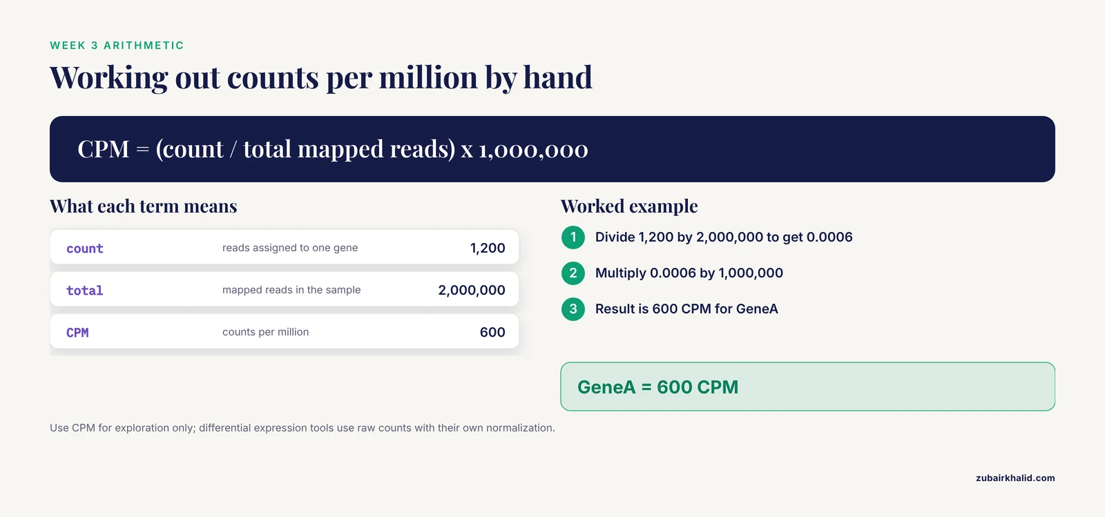
Week 3 introduces counts per million, the simplest normalization. The formula is CPM equals the count assigned to a gene divided by total mapped reads, multiplied by 1,000,000. Worked example: GeneA receives 1,200 reads in a sample with 2,000,000 mapped reads, so 1,200 divided by 2,000,000 equals 0.0006, and 0.0006 times 1,000,000 equals 600 CPM. Use CPM for exploration. Differential expression tools use raw counts with their own normalization, which is the point of week 4.
Week 4 uses a small shared count table, data/counts.csv:
gene,ctrl_1,ctrl_2,ctrl_3,trt_1,trt_2,trt_3
GeneA,1200,1100,1250,2400,2600,2550
GeneB,300,280,310,290,305,285
GeneC,50,45,55,48,52,47
And the script, sessions/week04_deseq.R:
library(DESeq2)

counts <- read.csv("data/counts.csv", row.names = 1)
meta <- data.frame(
  row.names = colnames(counts),
  condition = c("ctrl", "ctrl", "ctrl", "trt", "trt", "trt")
)

dds <- DESeqDataSetFromMatrix(countData = counts, colData = meta, design = ~ condition)
dds <- DESeq(dds)
res <- results(dds, contrast = c("condition", "trt", "ctrl"))
summary(res)
The parameters that matter: design = ~ condition tells the model to explain counts as a function of the condition column, and the contrast argument lists factor then reference level, so results are computed as treated versus control. results() by default applies a 0.1 cutoff on adjusted p-values and performs independent filtering of low-count genes. Adjusted p-values exist because testing thousands of genes at once manufactures false positives, and the Benjamini-Hochberg procedure controls the false discovery rate, which is the expected proportion of false positives among your called significant genes. On a run against this toy table, summary(res) prints lines in this shape, with your own numbers:
out of 3 with nonzero total read count
adjusted p-value < 0.1
LFC > 0 (up)    : 1, 33%
LFC < 0 (down)  : 0, 0%
Read those lines aloud in the meeting. Up means positive log2 fold change, the log ratio of expression between conditions. Week 5 then plots them:
library(ggplot2)

df <- as.data.frame(res)
df$gene <- rownames(df)
ggplot(df, aes(x = log2FoldChange, y = -log10(padj))) +
  geom_point() +
  theme_minimal()
ggsave("results/volcano.png", width = 5, height = 4)
Week 6 turns the group outward. Pick a published analysis and reproduce its simplest figure. A systematic review of microRNA signatures in atrial fibrillation pooled 40 articles, distilled 283 reported dysregulated microRNAs (short noncoding RNAs that regulate gene expression) down to 51 with a consistent direction of change, and flagged miR-223-3p as the most upregulated [9]. A figure of that kind, a table or a direction-consistent bar chart, is a realistic reproduction target. Nobody redoes a docking calculation in week 6, and saying so out loud keeps expectations honest. Groups without count data can run a sequence-flavored week instead, pulling protein entries from UniProt and computing simple composition statistics in the spirit of published viral protein characterizations [5].
Step 6: Run meetings people keep attending
Rotate the driver every week. The driver shares a screen and types, everyone else follows in their own terminal and calls out corrections. Nobody lectures, ever. The fastest failure mode for a study group is turning into a seminar series where one confident person talks and five people quietly stop coming.
Keep three artifacts alive. The debug log in notes/ collects every error message and its fix, dated, and becomes the group's internal FAQ within a semester. The session plans in sessions/ make week 7 writable by a member who missed week 3. The charter absorbs disputes before they become drama, because the decision rule is already written down.
Hold the timebox. Ninety minutes means ninety minutes, and ending on time is the single cheapest retention tool you have. Homework always produces a committed file, which gives the recap minute something concrete to review. Pair novices with experienced members for homework, and let the pairs swap every fortnight.
For remote and hybrid meetings, one shared screen is the room. Everyone else runs the same commands locally and pastes errors into chat. If more than one person is typing on the shared machine, stop and switch to follow-along mode, because merged typing destroys the very debugging skill the group exists to build.
Step 7: Close the season with a deliverable
Week 12 ends with an artifact, not a feeling. The minimum deliverable is one reproduced figure plus a README that records software versions, the environment file, and every command in order. Present it internally, then offer it to a department seminar or a campus poster session if the group wants an audience.
Then hold a thirty-minute retrospective and decide whether to renew. Renewal usually means a new track with the same format and the same repository, which is exactly how the infrastructure investment pays off. Groups that document their pipelines well can also absorb new members without restarting, and can widen scope deliberately, for example from plain differential expression toward the network and docking methods that integrative papers stack on top of it.
Common Mistakes and Limitations
- Scope creep. A group that decides to "learn bioinformatics" learns nothing by December. One track, one deliverable, one season. Add a second track only after the first deliverable exists.
- Environment drift. The moment members install packages ad hoc, results diverge and trust evaporates. Every new tool enters through the pinned environment file and a commit, never through a random
pip installin a base environment. - Lecture mode. If nobody typed during the meeting, the meeting failed. Keep the driver rotating and the hands-on block sacred.
- Starting with real production data. A 40-gigabyte metagenome will stall every laptop in the room. Subset the data or use synthetic data until the pipeline works end to end, then scale up once.
- Ignoring design and controls. Omics conclusions are only as good as the design behind them, which is why practical guides for non-specialists spend their early pages on negative and positive controls and on sample size before any code appears [2]. A study group that skips this produces analysts who can run pipelines on meaningless experiments.
- Overtrusting convenient servers. Web servers for survival and prognostic analysis are genuinely useful for quick hypothesis generation, but the same review literature notes that very few prognostic biomarkers reach clinical practice, largely because of missing independent validation [4]. Treat every server hit as a hypothesis with a mandatory caveat list.
- Underestimating reproduction. Published analyses omit versions, parameters, and sometimes steps. Budget a full session for what the paper describes in one sentence, and treat a partial reproduction with documented deviations as success.
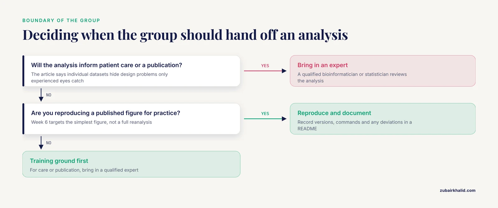
- The boundary of a study group. This format is a training ground. For analyses that will inform patient care or carry a publication, bring in a qualified bioinformatician or statistician, because individual datasets routinely hide design problems that only experienced eyes catch.
Frequently Asked Questions
How many people do I need to start a bioinformatics study group?
Four to eight people is the practical sweet spot, and three is enough to begin. Small groups let everyone present within a month, debug together on one shared screen, and survive a couple of dropouts without collapsing.
Do I need to be an expert to start a bioinformatics study group?
No. The organizer's job is logistics: booking the room, maintaining the repository, and keeping the rotation moving. Expertise rotates in through the presenter role, and half of every session is members discovering what nobody in the room knows.
What happens in a typical session?
Ninety minutes split into a recap, a 45-minute hands-on block with one driver sharing a screen, a troubleshooting circle where every error goes into a debug log, and a closing five minutes that assigns homework and confirms the next driver.
How is a study group different from a bioinformatics course?
A course supplies a graded syllabus and expert instruction, while the group supplies accountability, live debugging, and adaptation to your own data. The strongest setup uses a course as the spine and the group for everything courses skip, mainly installation, errors, and judgment calls.
Can we run the group fully remote?
Yes. You need a video call, one shared screen, a repository everyone can push to, and the discipline that members run commands on their own machines rather than watching. Hybrid works too, provided remote members get the same screen and audio quality as the room.
What should we install before the first meeting?
A package manager (Miniconda), git, and a text editor. Everything else should come from the group's pinned environment file, so that the first meeting starts with identical software on every laptop instead of forty minutes of individual installation attempts.
How long should a bioinformatics study group run?
Plan a 12-week season with an explicit deliverable in week 12, then decide in a retrospective whether to renew with a new track. Open-ended groups decay, while seasons with endings produce artifacts and clean stopping points.
What if members have very different skill levels?
Pair experienced members with beginners for homework, give tiered tasks (novices run commands, experienced members modify them), and let advanced members prepare sessions rather than dominate them. Uneven rooms are normal, and the rotation converts the gap into teaching capacity rather than resentment.
Sources
- Recent trends on omics and bioinformatics approaches to study SARS-CoV-2: A bibliometric analysis and mini-review
- A guide to human microbiome research: study design, sample collection, and bioinformatics analysis
- A review of bioinformatics platforms for comparative genomics. Recent developments of the EDGAR 2.0 platform and its utility for taxonomic and phylogenetic studies.
- Comprehensive Review of Web Servers and Bioinformatics Tools for Cancer Prognosis Analysis
- Bioinformatics study of the DNA and RNA viruses infecting plants and bacteria that could potentially affect animals and humans
- Cardiovascular adverse events in chronic myeloid leukemia patients treated with nilotinib or imatinib: A systematic review, meta-analysis and integrative bioinformatics analysis
- Current Consensus for Rehabilitation Protocols of the Surgically Repaired Acute Mid-Substance Achilles Rupture: A Systematic Review and Recommendations From the "GAIT" Study Group.
- [ESCMID Study Group for Infections in Compromised Hosts (ESGICH) Consensus Document on the safety of targeted and biological therapies: an infectious diseases perspective (Soluble immune effector molecules [I]: anti-tumor necrosis factor-α agents).](https://pubmed.ncbi.nlm.nih.gov/29459143/)
- MicroRNA expression signatures of atrial fibrillation: The critical systematic review and bioinformatics analysis