How to Use Spot Instances for Bioinformatics Workloads
By Dr. Zubair Khalid, DVM, MS, PhD ·
By the end of this guide you will be able to check live spot prices from the command line, launch an interruptible instance safely, wire a Nextflow or AWS Batch pipeline so that reclaimed capacity costs you minutes instead of days, and verify both the scientific output and the bill. The commands use AWS as the main example because it dominates published cloud bioinformatics case studies, but the same design principles apply to Google Cloud preemptible VMs and to any provider that sells interruptible capacity at a discount.
Here is what you need on hand before starting:
- An AWS account with IAM permissions for EC2, S3, Batch, and Cost Explorer
- AWS CLI version 2 installed and configured (
aws, versionandaws configure) - A Nextflow pipeline (or a WDL workflow for Cromwell) that runs at least one sample end to end on an on-demand instance
- An S3 bucket in the region where you plan to compute, for reference data, intermediates, and results
- Docker or Singularity container images for your tools, so any replacement instance can resume identical software
What Spot Instances Are and Why Genomics Teams Use Them
A spot instance is spare cloud compute capacity that the provider sells at a steep discount and can reclaim when it needs the hardware back. On AWS, a reclaimed spot instance receives a two-minute interruption notice before termination. On Google Cloud, the equivalent product is called a Spot VM, historically known as a preemptible VM. The economic trade is simple. You pay far less per hour, and in exchange the provider may take the machine away at any time.
For genomics, that trade is usually excellent. Most sequencing analysis is embarrassingly parallel, meaning it splits into thousands of independent tasks that never talk to each other. A whole genome pipeline processes one sample per shard. An RNA-seq quantification processes one library per shard. Published case studies show how much this matters in practice.
A tick genomics study assembled the large and repetitive genomes of two cattle tick species, Rhipicephalus microplus and R. appendiculatus, from Oxford Nanopore data using Shasta, and finalized the assemblies on AWS while capitalizing on spot discounts of up to 90 percent, producing draft genomes comparable to published tick genomes that relied on far more expensive infrastructure [1]. Falco, a cloud framework for single-cell RNA-seq processing built on Apache Hadoop and Spark, used AWS spot instances for its worker nodes and achieved roughly a 65 percent reduction in analysis cost while running 2.6 to 145.4 times faster than a standalone optimized machine [2]. A study that quantified transcript expression for 12,307 RNA-seq samples from the Cancer Cell Line Encyclopedia and The Cancer Genome Atlas processed samples on preemptible VMs for as little as $0.09 per sample [3]. And a medical imaging project that ran AI segmentation over 126,000 CT volumes used more than 21,000 virtual machines to finish in under 9 hours, work that would have taken an estimated 522 days on a single workstation, for a total compute cost of $1,011.05 [4]. The same massive-shard pattern applies directly to cloud bioinformatics.
The savings are not a trick of one study. A cost and scalability analysis of whole genome association studies on Spark clusters found consistent speed-versus-cost compromises across both Google Cloud Platform and Amazon Web Services, meaning the economics of elastic, interruptible compute hold up across providers [5]. Cost-aware schedulers have been built specifically to exploit this, including Aether, which uses linear programming to bid optimally on combinations of underutilized cloud resources for genomic analysis [6].
Which Bioinformatics Workloads Fit Spot, and Which Do Not
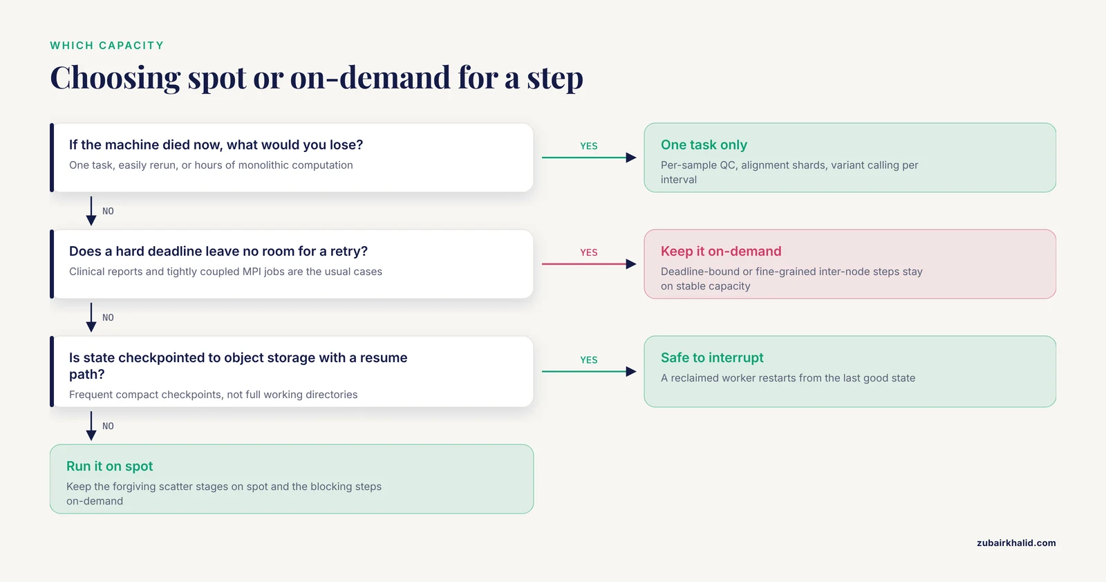
The single question that decides everything is this: if the machine vanished right now, what would you lose?
Use spot instances when the answer is "one task, easily rerun." This covers the large majority of AWS genomics and general cloud bioinformatics work:
- Per-sample QC, trimming, and alignment shards
- Variant calling where each shard handles one chromosome, one sample, or one genomic interval
- RNA-seq quantification and pseudoalignment per library
- Distributed Spark or Hadoop analytics, where the framework itself re-executes lost partitions
- Array jobs that fan out over hundreds of similar tasks
- Embarrassingly parallel image segmentation and feature extraction over large cohorts [4]
Approach with caution and heavy checkpointing when the answer is "hours of monolithic computation." Genome assembly is the classic case. Some assemblers hold the entire graph in memory for the whole run. Yet even assembly has been done successfully on spot capacity. The tick genome study ran Nanopore-only assembly through Shasta on AWS spot instances and published competitive draft genomes [1]. The general pattern that makes this survivable is frequent checkpointing of assembly state to object storage, plus a resume mechanism that restarts from the last good state rather than from zero.
Avoid spot for work where an interruption is genuinely unrecoverable or where a hard deadline leaves no room for a retry. A tightly coupled MPI job with fine-grained inter-node communication degrades badly if one node dies mid-step. A clinical pipeline that must return a report in a fixed window is better served by on-demand capacity with spot used for the forgiving scatter stages around it. The clinical NGS workflow GenomeKey was benchmarked specifically for turnaround time and cost, and its optimization insights centered on strategic batching of genomes and cluster configuration, which is exactly the kind of tuning you want before adding interruption risk to a clinical path [7].
One more consideration is data gravity. Public data compendia are now measured in petabytes, which makes transferring them to local machines infeasible and pushes analysis toward running compute where the data lives [3]. The same logic applies at smaller scale. Keep your reference files, intermediates, and results in the same region as your spot fleet so that every reclaimed worker rehydrates from fast local storage rather than a cross-region transfer.
Using Spot Instances for Bioinformatics Workloads Step by Step
This walkthrough builds a small, interruption-safe cohort analysis. The commands are real AWS CLI. Where output is shown, prices and identifiers are illustrative examples. Always read live values from your own account.
Step 1. Check current spot prices for candidate instance types
Spot prices fluctuate by instance family, size, and availability zone. Never launch on folklore. Query the history:
aws ec2 describe-spot-price-history \
  --region us-east-1 \
  --instance-types c6i.4xlarge m6i.4xlarge r6i.4xlarge \
  --product-description "Linux/UNIX (Amazon VPC)" \
  --start-time $(date -u -d "2 days ago" +%Y-%m-%dT%H:%M:%SZ) \
  --query 'SpotPriceHistory[].{Type:InstanceType,AZ:AvailabilityZone,Price:SpotPrice}' \
  --output table
Expected output (example values, yours will differ):
------------------------------------------------------------
|               DescribeSpotPriceHistory                   |
+---------------------+------------------------+-----------+
|        Price        |      AvailabilityZone  |   Type    |
+---------------------+------------------------+-----------+
|  0.2398             |  us-east-1a            | c6i.4xlarge|
|  0.2611             |  us-east-1b            | c6i.4xlarge|
|  0.2984             |  us-east-1a            | r6i.4xlarge|
|  0.2520             |  us-east-1c            | m6i.4xlarge|
+---------------------+------------------------+-----------+
Two habits matter here. First, compare the spot price to the on-demand price for the same type. If the discount is thin, on-demand may cost barely more and eliminates interruption risk for that task. Second, notice that prices differ between availability zones within the same region. Zone-level price spread is normal and is one reason to diversify.
Step 2. Score availability before committing
Historical prices tell you about the past. Spot placement scores tell you about the present. They estimate how likely AWS is to actually fulfill your requested capacity right now:
aws ec2 get-spot-placement-scores \
  --region us-east-1 \
  --instance-types c6i.4xlarge m6i.4xlarge r6i.4xlarge \
  --target-capacity 480 \
  --target-capacity-unit-type vCPU \
  --output json
Expected output (example):
{
  "SpotPlacementScores": [
    {
      "Region": "us-east-1",
      "AvailabilityZoneId": "use1-az2",
      "Score": 9
    },
    {
      "Region": "us-east-1",
      "AvailabilityZoneId": "use1-az4",
      "Score": 7
    }
  ]
}
Scores run from 1 to 10, where higher means a better chance of getting and keeping the capacity. A score of 9 for a target of 480 vCPUs, which is 30 c6i.4xlarge instances, says the region can absorb your cohort. A low score across every zone is a signal to widen your instance pool or shift the run to a quieter window.
Step 3. Launch a single spot worker and confirm its lifecycle
Launch one machine to validate your image, your IAM role, and your storage mounts before scaling:
aws ec2 run-instances \
  --region us-east-1 \
  --image-id ami-0123456789abcdef0 \
  --instance-type c6i.4xlarge \
  --key-name bio-key \
  --security-group-ids sg-0123456789abcdef0 \
  --subnet-id subnet-0123456789abcdef0 \
  --iam-instance-profile Name=genomics-worker-role \
  --block-device-mappings '[{"DeviceName":"/dev/xvda","Ebs":{"VolumeSize":200,"VolumeType":"gp3","DeleteOnTermination":false}}]' \
  --instance-market-options '{"MarketType":"spot","SpotOptions":{"MaxPrice":"0.68","SpotInstanceType":"one-time","InstanceInterruptionBehavior":"terminate"}}' \
  --tag-specifications 'ResourceType=instance,Tags=[{Key=Name,Value=spot-align-worker},{Key=pipeline,Value=wgs-qc}]' \
  --query 'Instances[].InstanceId' --output text
Expected output:
i-0abc123def4567890Setting DeleteOnTermination to false on the root volume means a reclaimed instance leaves its disk behind for inspection, which is invaluable the first time something fails mysteriously. Confirm the machine actually came up as spot:
aws ec2 describe-instances \
  --region us-east-1 \
  --instance-ids i-0abc123def4567890 \
  --query 'Reservations[].Instances[].{ID:InstanceId,Lifecycle:InstanceLifecycle,State:State.Name}' \
  --output json
Expected output:
[
  {
    "ID": "i-0abc123def4567890",
    "Lifecycle": "spot",
    "State": "running"
  }
]
If Lifecycle says spot, you are paying the spot rate. If the launch fails instead, the two most common errors are AuthFailure or UnauthorizedOperation, which mean your IAM user lacks ec2:RunInstances on the AMI or subnet, and InsufficientInstanceCapacity, which means that specific type and zone is full. Fix the first by correcting the policy. Fix the second by trying another zone or instance size from your Step 1 list.
Step 4. Make the workload interruption-safe
This step is the heart of using spot instances for bioinformatics. Three rules, in order of importance.
Rule one, all intermediates live on object storage or a shared filesystem that outlives any single machine. Never rely only on the instance store or an ephemeral EBS volume that dies with the machine. In Nextflow, point the work directory at S3:
// nextflow.config
workDir = 's3://mylab-genomics/work'

process {
  executor          = 'awsbatch'
  queue             = 'spot-ce-queue'
  errorStrategy     = 'retry'
  maxRetries        = 3
  cpus              = 16
  memory            = '64 GB'
}

aws {
  region = 'us-east-1'
  batch {
    cliPath              = '/usr/local/bin/aws'
    maxParallelTransfers = 16
    maxTransferAttempts  = 5
  }
}
Rule two, enable resume so a restarted pipeline skips everything that already finished. Nextflow's -resume flag hashes each completed task and reuses its cached outputs. When a spot instance dies after task 40 of 120, the restart redoes 80 tasks instead of 120:
nextflow run main.nf \
  -profile awsbatch \
  -resume \
  -with-report report.html
Expected output on a resumed run:
Cached process > ALIGN :SAMPLE_07
Cached process > ALIGN :SAMPLE_08
Submitted process > CALL Variants (SAMPLE_09)
Submitted process > CALL Variants (SAMPLE_10)
...
Pipeline completed successfully, with 88 of 120 processes cached
Rule three, listen for the interruption notice. AWS writes an instance-action document to the instance metadata endpoint two minutes before reclaiming the machine. A small watchdog loop on each worker can flush state during that window:
#!/usr/bin/env bash
TOKEN=$(curl -s -X PUT "http://169.254.169.254/latest/api/token" \
  -H "X-aws-ec2-metadata-token-ttl-seconds: 300")

while true
do
  ACTION=$(curl -s -H "X-aws-ec2-metadata-token: $TOKEN" \
    http://169.254.169.254/latest/meta-data/spot/instance-action)
  if [ -n "$ACTION" ]
  then
    echo "Interruption notice: $ACTION"
    aws s3 sync ./results s3://mylab-genomics/checkpoints/$SAMPLE_ID/ --quiet
    exit 0
  fi
  sleep 20
done
Expected output when the notice arrives:
Interruption notice: {"action":"terminate","time":"2026-11-11T15:30:00Z"}Two minutes is enough to upload a few gigabytes of compressed state, not enough to upload a terabyte of raw intermediates. Design checkpoints accordingly, saving compact state objects rather than full working directories.
Step 5. Scale with AWS Batch on a spot compute environment
For cohorts, let a scheduler manage spot instead of hand-launching instances. AWS Batch has a dedicated spot compute resource type with its own allocation strategy. Create the compute environment:
aws batch create-compute-environment \
  --region us-east-1 \
  --compute-environment-name spot-ce \
  --type MANAGED \
  --state ENABLED \
  --compute-resources '{
    "type": "SPOT",
    "allocationStrategy": "SPOT_CAPACITY_OPTIMIZED",
    "bidPercentage": 90,
    "minvCpus": 0,
    "maxvCpus": 512,
    "instanceTypes": ["c6i", "m6i", "r6i"],
    "instanceRole": "arn:aws:iam::123456789012:instance-profile/ecsInstanceRole",
    "subnets": ["subnet-0123456789abcdef0"],
    "securityGroupIds": ["sg-0123456789abcdef0"]
  }'
Expected output:
{
  "computeEnvironmentName": "spot-ce",
  "computeEnvironmentArn": "arn:aws:batch:us-east-1:123456789012:compute-environment/spot-ce"
}
The two parameters that matter most are allocationStrategy and bidPercentage. SPOT_CAPACITY_OPTIMIZED pulls from whichever of your listed pools currently has the deepest spare capacity, which reduces interruptions compared with chasing the absolute lowest price. bidPercentage of 90 caps your payment at 90 percent of the on-demand rate. Check that the environment came up valid:
aws batch describe-compute-environments \
  --region us-east-1 \
  --compute-environments spot-ce \
  --query 'computeEnvironments[].{Name:computeEnvironmentName,Status:status,Reason:statusReason}' \
  --output table
Expected output:
|DescribeComputeEnvironments               |
+------+-------+---------------------------+
| Name | Status|       statusReason        |
+------+-------+---------------------------+
|spot-ce| VALID |  ComputeEnvironment healthy|
+------+-------+---------------------------+
A status of INVALID with a reason mentioning the bid percentage means your cap is below what the market will currently bear. Raise bidPercentage toward 100, or widen the instance pool, then update the environment.
Step 6. Worked cost calculation
Compute the bill before the run, using live prices from Step 1. Example figures, illustrative only:
Per-sample work:        16 vCPUs x 6 hours     = 96 vCPU-hours
Cohort:                 30 samples x 96        = 2,880 vCPU-hours

c6i.4xlarge on-demand   = $0.68 per instance-hour
                        = $0.0425 per vCPU-hour
On-demand cohort cost   = 2,880 x $0.0425      = $122.40

c6i.4xlarge spot        = $0.24 per instance-hour
                        = $0.015 per vCPU-hour
Spot cohort cost        = 2,880 x $0.015       = $43.20

Savings                 = (122.40 - 43.20) / 122.40 = 64.7%
That 65 percent figure is not cherry-picked. Falco reported approximately a 65 percent cost reduction from spot workers on real single-cell RNA-seq pipelines [2], and the tick assembly study exploited discounts of up to 90 percent on AWS [1]. Your realized number depends on region, family, and the intensity of demand when you launch.
Add an interruption budget to the calculation. If roughly 5 percent of task-hours are lost and redone, multiply spot cost by 1.05. Even with that tax, interruptible capacity usually wins for scatter-heavy genomics.
Step 7. Verify the result is actually right
Spot introduces failure modes, so verification is not optional.
First, scientific verification. Run one sample end to end on an on-demand instance and once on a spot instance with the same container image and parameters. Compare outputs:
aws s3 cp s3://mylab-genomics/results/sample01/calls.vcf.gz . \
  --expected-md5-hash-of-content $(md5sum spot_run.vcf.gz | cut -d' ' -f1)
Or, more simply, hash both copies locally with md5sum and confirm the digests match. Deterministic pipelines should produce bit-identical results regardless of the hardware they ran on. If they differ, your pipeline depends on something environment-specific, which is a bug worth finding before spot ever interrupts anyone.
Second, operational verification. Check how many interruptions your run absorbed:
aws ec2 describe-spot-instance-requests \
  --region us-east-1 \
  --query 'SpotInstanceRequests[].{State:State,Status:Status.Code}' \
  --output table
Expected output:
|DescribeSpotInstanceRequests|
+-------------+---------------+
|    State    |     Status    |
+-------------+---------------+
|   active    | fulfilled     |
|   active    | fulfilled     |
|   active    | fulfilled     |
+-------------+---------------+
Interruption events also appear in CloudTrail and CloudWatch, which is where you build the report for your next grant application. Third, financial verification. In the AWS console, activate cost allocation for the pipeline tag, then check Cost Explorer filtered on that tag. Tagging every resource in Step 3 is what makes this possible. Studies of cloud cost structure, such as the Atlas2 Cloud personal genome pipeline, broke billing into storage, compute, and I/O components precisely so that cost could be attributed and tuned per stage [8]. Build that habit from day one.
Key Spot Settings at a Glance
| Setting | What it controls | Recommended practice for genomics |
|---|---|---|
| Allocation strategy | Which spare-capacity pool Batch or a fleet draws from | SPOT_CAPACITY_OPTIMIZED for Batch, capacity-optimized for fleets |
bidPercentage | Maximum percentage of on-demand price you will pay | 90 to 100. Lower caps rarely fill and cause INVALID environments |
| Instance pool width | Number of families and sizes available | 3 to 5 current-generation families, for example c6i, m6i, r6i, plus Graviton variants |
InstanceInterruptionBehavior | What happens at reclaim time | terminate, with all state checkpointed to S3 or GCS beforehand |
| Max price | Hourly ceiling for raw EC2 spot requests | Leave at the on-demand default unless you model bids explicitly, as Aether does with linear programming [6] |
| Work directory | Where intermediates live | Object storage such as S3, never instance store alone |
| Retry policy | Behavior after a failed task | Retry up to 3 times with checkpoint resume enabled |
| Checkpoint granularity | How much work a single interruption destroys | Checkpoint per pipeline step or per chunk, not per hour of runtime |
Workflow Managers and Distributed Frameworks on Spot
Modern workflow managers are the practical reason spot instances for bioinformatics work at all. They convert a brittle single-machine run into a resumable DAG of stateless tasks, which is exactly the shape spot capacity rewards.
Nextflow is the current default for AWS genomics pipelines. Its combination of -resume, S3-backed work directories, and the awsbatch executor covers everything in Steps 4 through 5. The key config discipline is errorStrategy = 'retry' paired with maxRetries, so that a task killed at the two-minute mark is requeued automatically rather than failing the whole run. Cromwell, the WDL engine behind several major genomics platforms, provides equivalent call-caching. Snakemake offers rerun-incomplete, which detects outputs left incomplete by a killed worker and re-executes just those rules.
For distributed frameworks, spot works differently and better. Spark and Hadoop re-execute lost partitions themselves, so losing a worker costs minutes, not the job. Falco demonstrated this directly, parallelizing established RNA-seq alignment and quantification pipelines over Spark with spot worker nodes [2]. Genome-wide association studies on Spark and Hail showed that the same analysis reached similar performance and cost sweet spots on both GCP and AWS, which gives you freedom to arbitrage spot capacity across providers [5]. Deep learning based variant calling has followed the same route, with DeepVariant-on-Spark deployed on Google Cloud to give researchers without local clusters a scalable path to GPU-assisted DeepVariant analysis [9].
Even core data primitives have been rewritten for this environment. A cloud-native distributed pileup implementation, SeQuiLa, cut execution time by up to 6.5 times and memory use by up to 2 times compared with other distributed tools, which the authors tied directly to substantial cloud cost reduction, and it deploys on managed Kubernetes and Hadoop services in public clouds [10]. When a pipeline bottleneck is a single expensive step, optimizing that step often buys more than aggressive spot bidding does.
Cost-aware scheduling on top of spot is its own discipline. Aether treats instance selection and bidding as a linear programming problem, minimizing total cost while keeping the user's existing HPC pipeline shape [6]. Workflow scheduling research on epigenomics pipelines found that an improved particle swarm optimization scheduler reduced total cost by 6.83 percent versus a standard particle swarm approach, a useful reminder that even small scheduling gains compound across thousands of tasks [11]. You do not need to implement any of these algorithms yourself. What you need is a manager that retries, a filesystem that survives, and enough instance diversity that the scheduler always has somewhere to place work.
Large institutional platforms make the same choices at scale. The UK Biobank Research Analysis Platform study that fine-mapped coronary artery disease loci reported a 44 percent cost reduction and a 94 percent speedup purely through compute architecture optimization on an existing managed platform [12], and the SenNet Data Portal runs on a scalable hybrid cloud microservices architecture supporting hundreds of multimodal datasets across contributing centers [13]. The pattern to copy is hybrid and layered. Keep a stable on-demand or reserved baseline for the steps that must never fail, and burst the parallelizable bulk onto spot.
Spot Instances Bioinformatics Tips
These tips are the difference between a spot setup that feels fragile and one that hums.
- Diversify the pool. Pick 3 to 5 current-generation families that meet your memory profile, for example c6i, m6i, r6i, and their Graviton equivalents. A pipeline pinned to a single instance type is one capacity event away from stalling, while a diversified pool lets the scheduler route around trouble. The cost-scalability study across AWS and GCP compared many cluster configurations precisely because different configurations behave differently under real conditions [5].
- Separate scatter from gather. Put the fan-out stages, which are usually 90 percent of the compute, on spot. Keep alignment of references, index building, joint genotyping of merged outputs, and any step that blocks the whole pipeline on one machine on on-demand or reserved capacity. This is the layering that institutional platforms converge on.
- Batch intelligently. How many samples go into one task changes both efficiency and blast radius. GenomeKey's benchmarking of clinical-scale whole genome analysis found that strategic batching of individual genomes was a key optimization lever for turnaround time and cluster configuration [7]. Fewer, larger tasks amortize container startup and transfer overhead. More, smaller tasks reduce the cost of any single interruption. Tune this per pipeline rather than by rule of thumb.
- Choose storage with the failure model in mind. Assemblers and graph workloads are I/O hungry. Research on cloud-based parallel assembly with GiGA found that an SSD-based private cloud infrastructure significantly outperformed a traditional HPC cluster [14]. On spot, where machines vanish, that points to NVMe instance store for scratch plus object storage for checkpoints, never instance store alone.
- Run the watchdog everywhere. Install the interruption-metadata loop from Step 4 into every worker image, not just the one you test. The one run you skip it on is the one that loses six hours of state.
- Price-check before every large run. Spot prices drift over weeks. The two-minute check in Step 1 occasionally reveals that a different family is now far cheaper for the same vCPU count, or that your region has tightened. Consider automated bidding optimizers if your volume justifies it, in the spirit of Aether's linear programming approach [6].
- Transfer efficiently. Moving data into and out of the cloud is a real cost line, not a footnote. Closha, a cloud workflow system for massive sequencing data, built a dedicated transfer component after finding conventional uploads too slow [15]. For most labs, the simpler discipline is the same one from the data-gravity discussion: keep data and compute in one region, compress intermediates, and delete stale work directories on a schedule.
- Track cost per sample, not cost per run. The $0.09-per-sample figure from the 12,307-sample transcript quantification study [3] is the right unit of measurement for planning. Per-sample costs let you extrapolate to next year's cohort before you commit, and they expose pipelines whose cost is dominated by fixed overhead rather than analysis.
Common Mistakes and Limitations
These are the errors that actually burn people, along with the exact symptoms to watch for.
Mistake 1. Building a single-instance-type pipeline. Symptom: the pipeline runs fine for weeks, then stalls for a day with InsufficientInstanceCapacity or a Batch compute environment that never scales up. Fix: list 3 to 5 families in your compute environment and let SPOT_CAPACITY_OPTIMIZED choose. Check placement scores before large runs, as in Step 2.
Mistake 2. Keeping intermediates on instance store. Symptom: an interruption deletes six hours of work, and the Nextflow log shows the work directory was on /mnt/scratch with no remote copy. Fix: workDir on S3, checkpoints on object storage, DeleteOnTermination false on root volumes during development.
Mistake 3. Setting MaxPrice artificially low to save more. Symptom: spot requests sit in pending forever, or Batch reports the compute environment INVALID because the bid percentage is below market. Fix: set the cap at or near on-demand and rely on capacity-optimized allocation. The spot discount already applies automatically. A low cap does not lower your price, it only disqualifies you from ever filling.
Mistake 4. No interruption handler. Symptom: task logs end mid-line, the instance is gone, and nothing was flushed. Fix: the Step 4 watchdog plus pipeline-level retries. A task killed at minute 118 of a 120-minute task with no checkpoint loses 118 minutes. The same task split into 12 chunks loses at most 10.
Mistake 5. Treating spot price history as a prediction. History tells you where prices were, not where they will be. Teams that build budgets on the assumption that today's spot rate holds are routinely surprised. Budget on the on-demand rate, treat spot savings as upside, and re-verify prices before each large run.
Mistake 6. Using spot for deadline-critical stages with no fallback. Symptom: a clinical report misses its window because the final joint genotyping step was queued behind a burst of interruptions. Fix: on-demand or reserved capacity for deadline-bound steps, spot for the forgiving bulk. This is the layering principle applied to risk rather than cost.
Mistake 7. Ignoring data transfer geography. Symptom: compute bills look wonderful while the S3 data transfer line quietly doubles the total. Fix: one region for data and compute, compressed intermediates, and regular cleanup. Cost-structure studies like Atlas2 Cloud's breakdown of storage, compute, and I/O [8] exist because teams kept being surprised by exactly this.
Mistake 8. Running GPU training without checkpointing. Deep learning components, including model-based variant callers, can run on interruptible capacity, and DeepVariant-on-Spark shows the framework path exists on GCP [9]. But a training loop that saves model state only at the end of a multi-day run is a spot catastrophe waiting to happen. Checkpoint model weights on a fixed interval to object storage.
Limitations to keep in mind. Spot capacity is not guaranteed capacity. Availability varies by region, family, and moment, and no scheduler eliminates that variance, it only mitigates it. Interruptible discounts differ across providers and change over time, so any specific percentage you read, including those cited here, describes one study at one time rather than a durable market constant. And for human genomic data, security and compliance review applies to any compute environment, interruptible or not, so involve your institutional review before moving identifiable data into the cloud.
Frequently Asked Questions
How much can I save with spot instances for bioinformatics workloads?
Savings depend on instance family, region, current demand, and how much of your pipeline you can safely make interruptible, so there is no single universal number. Published genomics case studies report large reductions, and the correct figure for your own run comes from comparing live spot prices against on-demand rates for your actual instance mix before you launch.
What happens when a spot instance is interrupted mid-pipeline?
AWS writes a notice to the instance metadata two minutes before reclaiming the machine, then terminates it. A well-built pipeline loses only the currently running task, requeues it through a retry policy, and resumes from cached results on a replacement worker, which is why checkpointing and resume support are prerequisites rather than extras.
Can I run genome assembly or other long, monolithic jobs on spot instances?
Yes, but only with deliberate checkpointing of intermediate state to persistent storage and a resume path that restarts from the last good state. Published assembly work, including Nanopore-only tick genome assembly finalized on AWS, succeeded on spot capacity using this pattern.
Do spot instances work with Nextflow, Cromwell, and AWS Batch?
Yes. Nextflow pairs -resume with S3 work directories and the awsbatch executor, Cromwell provides equivalent call caching for WDL workflows, and AWS Batch offers a spot compute resource type with capacity-optimized allocation. These tools exist largely to make interruptible capacity practical for genomics.
How many instance types should I keep in my spot pool?
Keep 3 to 5 current-generation families that meet your memory and CPU profile, such as c6i, m6i, and r6i plus compatible Graviton variants. Diversity lets the scheduler route around capacity shortages in any single pool and materially reduces interruption impact.
Should I set a MaxPrice below the on-demand rate to save even more?
Generally no. A bid below the current market rate simply fails to fill or gets reclaimed more often, while the standard spot discount already delivers the savings automatically. Keep the cap at the on-demand default and rely on allocation strategy for cost and stability.
Can I use spot GPUs for deep learning in genomics?
Yes, provided your training loop checkpoints model weights to object storage on a regular interval. Framework-based approaches that distribute model training and inference across cloud clusters have been demonstrated for variant calling on Google Cloud, and the same interruption-safety rules apply as for CPU workloads.
Are spot instances appropriate for clinical genomic pipelines with hard deadlines?
For the parallel bulk stages, often yes. For deadline-bound or regulated steps with no tolerance for retry delays, use on-demand or reserved capacity and reserve spot for the forgiving surrounding work. Any clinical or regulated deployment also requires your institution's security and compliance review before identifiable data enters the cloud.
Sources
- Tick genomics through a Nanopore: a low-cost approach for tick genomics.
- Falco: a quick and flexible single-cell RNA-seq processing framework on the cloud.
- A cloud-based workflow to quantify transcript-expression levels in public cancer compendia.
- Cloud-based large-scale curation of medical imaging data using AI segmentation.
- Scalability and cost-effectiveness analysis of whole genome-wide association studies on Google Cloud Platform and Amazon Web Services.
- Aether: leveraging linear programming for optimal cloud computing in genomics.
- Scalable and cost-effective NGS genotyping in the cloud.
- Atlas2 Cloud: a framework for personal genome analysis in the cloud.
- DeepVariant-on-Spark: Small-Scale Genome Analysis Using a Cloud-Based Computing Framework.
- Cloud-native distributed genomic pileup operations.
- Cancer Diagnosis Epigenomics Scientific Workflow Scheduling in the Cloud Computing Environment Using an Improved PSO Algorithm.
- Optimizing UK biobank cloud-based research analysis platform to fine-map coronary artery disease loci in whole genome sequencing data.
- SenNet Portal: Build, Optimization and Usage.
- Large-scale parallel genome assembler over cloud computing environment.
- Closha: bioinformatics workflow system for the analysis of massive sequencing data.