How to Build a Single-Cell RNA-seq Analysis Pipeline in Nextflow
By Dr. Zubair Khalid, DVM, MS, PhD ·

By the end of this article you will be able to assemble a working single-cell RNA-seq analysis pipeline in Nextflow that takes raw 10x Chromium FASTQ files through read quality control, reference preparation, barcode and UMI counting, aggregate QC reporting, and a first pass at downstream cell-level analysis in Python. You will also know how to run it on a laptop or a SLURM cluster, resume interrupted runs, containerize every tool, and diagnose the errors that most often stop these pipelines.
To follow the walkthrough you need Java 17 or later, about 10 GB of free disk space, one of Docker, Apptainer, or Conda (or Mamba), and a test FASTQ pair from a droplet-based single-cell library. Everything shown here uses free, open-source tools and works on a standard laptop for small test datasets.
Why Nextflow for single-cell RNA-seq
Single-cell datasets break the habits that work for bulk sequencing. One experiment can contain hundreds of thousands of cells, libraries arrive in dozens of FASTQ files, and the analysis splits naturally into independent per-sample tasks followed by a collective downstream step. A workflow engine handles the bookkeeping so you do not have to.
Three properties make Nextflow the standard choice for this workload:
- Portability. A pipeline written once runs on a laptop, an HPC scheduler, or a cloud batch system with a profile switch. The nf-core community builds its pipelines on this foundation, and the scnanoseq pipeline for long-read single-cell RNA-seq cites portability, scalability, and reproducibility across runs as the reasons it is implemented in Nextflow on the nf-core framework [1].
- Modularity. Nextflow DSL2 lets you write each analysis step as an independent process with defined inputs and outputs, then swap modules without touching the rest of the code. The scAN1.0 pipeline for 10x data used this property to evaluate different genome mapping steps while keeping everything else fixed [2].
- Proven scalability at atlas scale. Benchmarking work encapsulated seven distinct high-throughput scRNA-seq processing pipelines in Nextflow and compared them across eight public datasets from five platforms, which shows both that the engine handles this data type and that it is a natural framework for evaluating alternative tools [3]. On the extreme end, the NEXT-scASV pipeline processes allele-specific variant calling from single-cell RNA-seq for atlas-level studies and demonstrated its design on 135,000 peripheral blood mononuclear cells from 57 donors [4].
The rest of this article shows you how to build a small but production-shaped pipeline of your own, then points you to established templates when you would rather adopt one.
Prerequisites and setup
Install Nextflow and verify the toolchain:
java -version
curl -s https://get.nextflow.io | bash
mv nextflow /usr/local/bin/
nextflow -v
Expected output of the last command:
nextflow version 24.04.0Next, install a container engine. Docker works on macOS and on most Linux workstations. On HPC systems where you lack root access, use Apptainer (formerly Singularity) or the Conda profile shown later. You do not need all three.
Finally, confirm you have a test dataset. Any paired-end FASTQ files from a droplet-based assay with a barcode-plus-UMI read structure will work. The walkthrough assumes 10x Genomics 3' chemistry, which is the most common starting point. Two definitions you will meet constantly:
- Cell barcode: a short sequence in read 1 that identifies which droplet (and therefore which cell) a read came from.
- UMI (unique molecular identifier): a short random sequence, also in read 1, that tags each original mRNA molecule so that PCR duplicates can be collapsed during counting.
Anatomy of a single-cell RNA-seq analysis pipeline
Every published single-cell pipeline, whether custom or framework-based, has the same spine. For example, scAN1.0 for 10x data and nf-core/scnanoseq for Nanopore long-read data both organize their work into barcode handling, alignment, UMI deduplication, quantification, and QC reporting, [1]. Your pipeline needs the following stages:
- Raw read QC. FastQC on every FASTQ file, aggregated later with MultiQC. This catches sequencing-level problems such as low quality tails or adapter contamination before you waste compute on counting.
- Reference preparation. Build or download a reference index and a transcript-to-gene mapping. Doing this as a pipeline task rather than a manual step is what makes the run reproducible on a new machine.
- Barcode and UMI processing plus counting. For short-read droplet data, the kallisto and bustools pair (
kb) performs barcode detection and correction, pseudoalignment to the transcriptome, UMI deduplication, and gene-level counting in one command. Long-read assays need different tools at this stage because the cell barcode and UMI must be extracted from full-length reads, which is exactly what the scnanoseq pipeline automates for Oxford Nanopore data [1]. - Per-sample QC on the count matrix. Mapping rates, valid barcode fractions, knee plots, and estimates of empty droplets.
- Downstream analysis. Cell filtering, normalization, dimensionality reduction, clustering, and annotation. This can live inside the pipeline as a script, or the pipeline can stop at the count matrix and hand off to R or Python.
The modular stage structure is also what makes the same skeleton reusable for related assays. FORGE reuses the pattern for single-nucleus multiome by running expression and accessibility branches and joining them for regulatory inference [5]. The single cell Advanced Chromatin Exploration pipeline couples scATAC-seq with scRNA-seq to derive cell-state-specific accessibility profiles [6]. BARtab applies it to synthetic lineage barcodes carried inside single-cell and spatial datasets [7]. Once your skeleton is right, the biology you swap in is a detail.
Pipeline format and project structure
A Nextflow project has a small, conventional layout. Learning this format once lets you read almost every pipeline published in the field, including every nf-core workflow [1].
scrnaseq-nf/
    main.nf
    nextflow.config
    environment.yml
    samplesheet.csv
    conf/profiles.config
    modules/fastqc.nf
    modules/kb_ref.nf
    modules/kb_count.nf
    modules/multiqc.nf
    assets/samplesheet_test.csv
The pieces have fixed jobs:
main.nfdeclares the workflow, the order of processes, and how data flows between them.modules/*.nfeach define one process. One tool, one file.nextflow.configholds parameters and process resource settings.conf/profiles.configholds execution profiles such as docker, conda, and slurm.environment.ymlpins the tool versions so that identical runs produce identical results.
If you prefer to start from a maintained template rather than an empty directory, the nf-core create command scaffolds a project with exactly this format, including test datasets, CI checks, and documentation. This is how most groups now start a custom pipeline.
Worked example: build the pipeline step by step
Step 1: Create the sample sheet
Nextflow pipelines should never hardcode file paths. Put them in a CSV instead. Create samplesheet.csv:
sample_id,fastq_1,fastq_2
pbmc_ctrl,pbmc_ctrl_S1_L001_R1_001.fastq.gz,pbmc_ctrl_S1_L001_R2_001.fastq.gz
pbmc_stim,pbmc_stim_S1_L001_R1_001.fastq.gz,pbmc_stim_S1_L001_R2_001.fastq.gz
The three columns are the minimum useful format for droplet data:
| Column | Meaning | Example |
|---|---|---|
sample_id | Label used for tagging, output folders, and reports | pbmc_ctrl |
fastq_1 | Read 1, containing cell barcode and UMI | ..._R1_001.fastq.gz |
fastq_2 | Read 2, containing the cDNA insert | ..._R2_001.fastq.gz |
Add columns as your needs grow, for example chemistry per sample or batch. Keep the header stable once tools depend on it.
Step 2: Pin the software environment
Create environment.yml so every tool version is fixed:
name: scrnaseq-kb
channels:
  - conda-forge
  - bioconda
dependencies:
  - kallisto =0.48.0
  - bustools =0.43.2
  - fastqc =0.12.1
  - multiqc =1.21
If you use Docker instead of Conda, build an image from the same file:
FROM mambaorg/micromamba:latest
COPY environment.yml /tmp/
RUN micromamba install -y -n base -f /tmp/environment.yml
One environment, two execution modes. This is the containerization strategy that published single-cell Nextflow pipelines use to make results reproducible across platforms [4], [2].
Step 3: Write the configuration
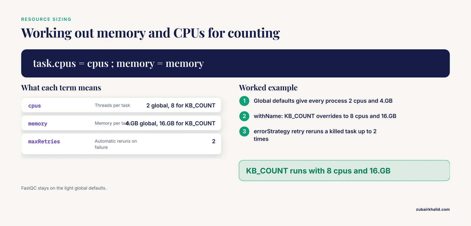
Create nextflow.config:
includeConfig 'conf/profiles.config'

params {
    samplesheet  = 'samplesheet.csv'
    outdir       = 'results'
    reference    = 'mouse'
    kb_chemistry = '10xv3'
}

process {
    conda         = "${projectDir}/environment.yml"
    cpus          = 2
    memory        = 4.GB
    errorStrategy = 'retry'
    maxRetries    = 2

    withName: KB_COUNT {
        cpus   = 8
        memory = 16.GB
    }
}
Create conf/profiles.config:
profiles {
    docker {
        docker.enabled = true
    }
    singularity {
        singularity.enabled = true
        singularity.autoMounts = true
    }
    conda {
        conda.enabled   = true
        conda.useMamba  = true
    }
    slurm {
        process.executor = 'slurm'
        process.queue    = 'batch'
    }
    test {
        params.samplesheet = "${projectDir}/assets/samplesheet_test.csv"
    }
}
Parameters that matter here:
errorStrategy = 'retry'withmaxRetries = 2makes transient failures, especially out-of-memory kills on counting tasks, rerun automatically. FORGE describes this interruption robustness as a design goal for cluster-based single-cell workflows [5].- The
withName: KB_COUNTblock overrides resources for the heaviest process only. Global defaults stay light for FastQC. - The
testprofile swaps in a small sample sheet so you can validate the pipeline in minutes before committing hours of cluster time.
Step 4: Write the modules
Each module is one process. Create modules/fastqc.nf:
process FASTQC {
    tag "${meta.id}"

    input:
    tuple val(meta), path(reads)

    output:
    tuple val(meta), path("*_fastqc.zip"), emit: zips
    path "*_fastqc.html", emit: htmls

    script:
    """
    fastqc ${reads}
    """
}
The tuple val(meta), path(reads) pattern is the standard DSL2 idiom: metadata travels with the data through every process, so each task knows its own sample name without relying on file names.
Create modules/kb_ref.nf:
process KB_REF {
    publishDir "${params.outdir}/reference", mode: 'copy'

    output:
    path "index.idx", emit: index
    path "t2g.txt", emit: t2g

    script:
    """
    kb ref -d ${params.reference} -i index.idx -g t2g.txt -f1 transcriptome.fa
    """
}
kb ref -d mouse fetches a standard preprocessed mouse transcriptome reference and builds the kallisto index plus a transcript-to-gene mapping. -d human does the same for human. If your organism is not in that set, point the process at your own FASTA and GTF instead and keep the same output names so the rest of the pipeline is unchanged.
Create modules/kb_count.nf:
process KB_COUNT {
    tag "${meta.id}"
    publishDir "${params.outdir}/counts/${meta.id}", mode: 'copy'

    input:
    tuple val(meta), path(reads)
    path index
    path t2g

    output:
    tuple val(meta), path("counts_unfiltered"), emit: counts

    script:
    """
    kb count \\
        -i ${index} \\
        -g ${t2g} \\
        -x ${meta.chemistry} \\
        -o counts_unfiltered \\
        -t ${task.cpus} \\
        ${reads}
    """
}
Key flags:
| Flag or parameter | Where it is set | What it controls | Sensible value |
|---|---|---|---|
-x | process script, fed from params.kb_chemistry | Barcode and UMI layout of the library | 10xv3 for 10x Chromium v3 |
-t | task.cpus | Threads for counting | 8 on a workstation |
-i, -g | passed from KB_REF | Reference index and transcript-to-gene map | Pipeline-managed |
-o | process script | Output directory for the unfiltered matrix | counts_unfiltered |
cpus / memory directives | nextflow.config | Resources per task | 8 CPUs and 16 GB for counting |
Create modules/multiqc.nf:
process MULTIQC {
    publishDir "${params.outdir}/multiqc", mode: 'copy'

    input:
    path reports

    output:
    path "multiqc_report.html", emit: report

    script:
    """
    multiqc ${reports}
    """
}
Step 5: Write the workflow
Create main.nf:
#!/usr/bin/env nextflow
nextflow.enable.dsl = 2

include { FASTQC   } from './modules/fastqc'
include { KB_REF   } from './modules/kb_ref'
include { KB_COUNT } from './modules/kb_count'
include { MULTIQC  } from './modules/multiqc'

workflow {

    reads = Channel
        .fromPath(params.samplesheet, checkIfExists: true)
        .splitCsv(header: true)
        .map { row ->
            meta = [id: row.sample_id, chemistry: params.kb_chemistry]
            tuple(meta, file(row.fastq_1, checkIfExists: true), file(row.fastq_2, checkIfExists: true))
        }

    KB_REF()
    KB_COUNT(reads, KB_REF.out.index, KB_REF.out.t2g)
    FASTQC(reads)
    MULTIQC(FASTQC.out.htmls.collect())
}
Three things deserve attention:
checkIfExists: trueon both the CSV and the FASTQ paths makes the pipeline fail fast, with a clear message, when a file is missing rather than failing an hour into counting.KB_COUNTconsumes the reads channel and bothKB_REFoutputs. Nextflow matches each sample with the correct index automatically.collect()gathers the per-sample FastQC HTML files into a single item for MultiQC. This is the standard way to turn per-sample work into a report step.
Step 6: Run the pipeline
nextflow run main.nf -profile conda -ansi falseExpected console output (task hashes will differ):
N E X T F L O W  ~  version 24.04.0
Launching `main.nf` [modest_curie] DSL2 - revision: 4a1b2c3d45
executor >  local (8)
[8f/3a1c20] KB_REF               | 1/1
[7d/f4b9aa] FASTQC (pbmc_ctrl)   | 2/2
[4a/91c2f3] KB_COUNT (pbmc_stim) | 2/2
[9b/2e7d55] MULTIQC              | 1/1
Completed at 11-Nov-2026 14:22 UTC (4m 51s) Duration: 4m 51s
The numbers after each process name show completed and total tasks. The two-character directory prefixes correspond to cached task directories under work/.
If you built the Docker image instead, run with -profile docker and add process.container to that profile so Nextflow knows which image to use.
Step 7: Resume after changes or interruptions
nextflow run main.nf -profile conda -resumeNextflow fingerprints every task on its inputs, the process script, and the container or environment. Tasks whose fingerprints are unchanged are pulled from cache and marked with a (cached) tag in the console output. Change one flag in KB_COUNT and only that process and its downstream steps rerun. This behavior is why pipeline authors can evaluate alternative tools inside a fixed pipeline, as scAN1.0 did when swapping mapping steps [2].
Step 8: Inspect the outputs
After a successful run, results/ contains:
results/
    reference/
        index.idx
        t2g.txt
        transcriptome.fa
    counts/pbmc_ctrl/counts_unfiltered/
    counts/pbmc_stim/counts_unfiltered/
    fastqc/
    multiqc/multiqc_report.html
Each counts_unfiltered directory holds the sparse count matrix and its barcode and gene name files (names resembling cells_x_genes.mtx, cells_x_genes.barcodes.txt, and cells_x_genes.genesnames.txt, with small variations between kb versions). Because the matrix is unfiltered, it contains every droplet, including empty ones. That is intentional and matters in the QC step below.
Step 9: Check the run is actually right
Do not trust a green completion line alone. Verify three layers:
- Sequencing-level QC. Open
multiqc_report.htmland confirm per-base quality, per-tail quality, and adapter content look healthy across all samples. A sample that drifts from the others here usually has a wet-lab explanation. - Counting-level QC. Inside each sample directory, kb writes summary metrics including the fraction of reads with a valid barcode, the fraction pseudoaligned, and barcode count distributions. For a healthy 10x v3 library at moderate depth you should see the large majority of reads assigned valid barcodes, a high pseudoalignment rate against a well-matched reference, and a knee plot with a clear separation between populated droplets and empty ones. A flat or unreadable knee plot is the classic sign of a failed or overloaded library.
- Biology-level sanity. Cell counts per sample should be in the same order of magnitude as the library design, and known marker genes should appear in the matrix.
From counts to cell types
A count matrix is not an analysis. The standard downstream chain, in Python with scanpy, reads the matrix, filters cells and genes, normalizes, finds variable genes, reduces dimensions, and clusters:
import scanpy as sc
import scipy.io as sio
import pandas as pd

counts_dir = "results/counts/pbmc_ctrl/counts_unfiltered"

X = sio.mmread(f"{counts_dir}/cells_x_genes.mtx").T.tocsr()
cells = pd.read_csv(f"{counts_dir}/cells_x_genes.barcodes.txt", header=None, sep="\t")
genes = pd.read_csv(f"{counts_dir}/cells_x_genes.genesnames.txt", header=None, sep="\t")

adata = sc.AnnData(X, obs=pd.DataFrame(index=cells), var=pd.DataFrame(index=genes))

sc.pp.filter_cells(adata, min_genes=200)
adata.var["mt"] = adata.var_names.str.startswith("MT-")
sc.pp.calculate_qc_metrics(adata, qc_vars=["mt"], percent_top=None, log1p=False, inplace=True)
adata = adata[adata.obs["pct_counts_mt"] < 15, :].copy()

sc.pp.normalize_total(adata, target_sum=1e4)
sc.pp.log1p(adata)
sc.pp.highly_variable_genes(adata, n_top_genes=2000)
sc.pp.pca(adata)
sc.pp.neighbors(adata)
sc.tl.leiden(adata)
adata.write("pbmc_ctrl_processed.h5ad")
The mitochondrial threshold of 15 percent is a reasonable working default for many tissues, but the right cutoff depends on the biology and should be set by looking at the distribution in your own data rather than copied blindly. In a Jupyter session you would follow this with sc.pl.violin on n_genes_by_counts, total_counts, and pct_counts_mt to choose your filters from the plots.
Clustering into discrete groups is only one way to read the data. Methods such as Stator label cells along several axes at once, resolving types into subtypes and states such as activation or cell cycle phase from higher-order gene expression dependencies, and ship their own Nextflow pipeline for exactly this step [8]. If your downstream question is about cell type proportions in tissue rather than in dissociated cells, spatial deconvolution methods such as cell2location and RCTD, which performed best in a benchmark of 11 methods that was itself made reproducible with a Nextflow pipeline [9], consume your scRNA-seq data as a reference.
Use a maintained template instead of writing your own
Writing the small pipeline above teaches you the format, but for production work you should strongly consider adopting an existing pipeline. The single cell rna-seq analysis pipeline nextflow template that most groups converge on is nf-core/scrnaseq, which supports multiple counting backends and follows the nf-core standards for testing, documentation, and containers [1]. To run it without writing any code:
nextflow run nf-core/scrnaseq -profile docker -r 1.3.0Parameter values go in a local config file rather than on the command line, which keeps your invocations short and version-controlled:
// my-config.config
params {
    input            = 'samplesheet.csv'
    outdir           = 'results'
    aligner          = 'kb'
    protocol         = '10xv3'
}
nextflow run nf-core/scrnaseq -profile docker -c my-config.configThe same logic applies beyond expression counting. When your assay adds a modality, look for a pipeline with the same shape before building one: FORGE for single-nucleus multiome [5], scnanoseq for long-read single-cell data [1], NEXT-scASV for allele-specific variant calling from 5' single-cell data [4], and BARtab plus the bartools R package for lineage barcoding [7].
Scaling to atlas-sized studies
Local profiles are for development. For real studies, add a scheduler profile and point Nextflow at your cluster:
profiles {
    slurm {
        process.executor   = 'slurm'
        process.queue      = 'batch'
        process.time       = '4h'
        process.memory     = '8 GB'
    }
}
Two practical notes for large runs:
- Per-sample processes parallelize across samples automatically because each item in the reads channel becomes an independent task. Atlas-scale projects work this way by design. NEXT-scASV, for example, highlights its modular design as what allows massive parallelization across a large cohort [4].
- Long runs will be interrupted. Restart with
-resume. Combining resume with a scheduler profile is what makes multi-day single-cell analyses tractable, and it is an explicit design feature of published cluster-oriented single-cell pipelines [5].
Troubleshooting guide
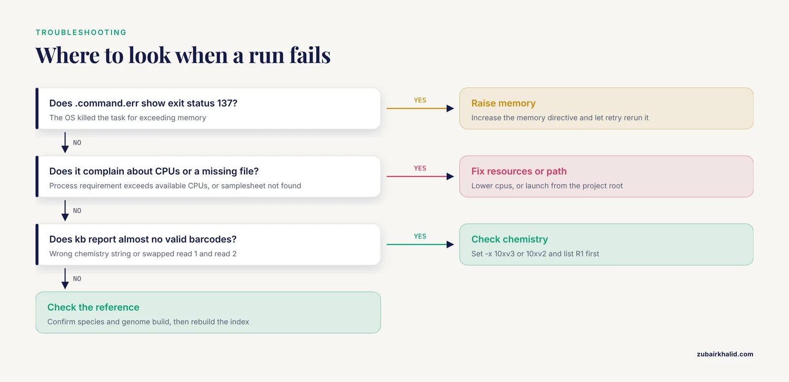
Most failures in a single-cell Nextflow pipeline fall into a handful of patterns. First, find the failed task and its real error output:
nextflow log -f process,exit_status
cat work/8f/3a1c20.../KB_COUNT/pbmc_ctrl/.command.err
Every task directory contains .command.sh (the exact script run), .command.err (stderr), and .command.out (stdout). Reading .command.err first resolves the majority of issues.
| Message or symptom | Likely cause | Fix |
|---|---|---|
Process KB_COUNT terminated with an error exit status (137) | The task was killed by the OS for exceeding memory | Raise the memory directive for that process and let errorStrategy = 'retry' rerun it |
Process requirement exceeds available CPUs | The process requests more cores than the machine or queue allows | Lower cpus for that process or submit to a queue with more cores |
No such file or directory: samplesheet.csv | Pipeline launched from the wrong directory or the parameter name is wrong | Launch from the project root or set params.samplesheet explicitly |
Fastq file not found: <path> from checkIfExists | A typo or missing file in the sample sheet | Correct the path, then rerun with -resume |
| kb reports almost no valid barcodes | Wrong chemistry string, or read 1 and read 2 are swapped | Confirm the kit version and set -x 10xv3 or 10xv2 accordingly, and confirm the R1 file is listed first |
| Pseudoalignment rate far below expectations | Reference does not match the sample or the genome build differs from the annotation | Verify species and genome build, rebuild the reference inside the pipeline |
docker: command not found when using the docker profile | Container engine missing or not in PATH | Install Docker or switch to the conda profile |
Beyond engine errors, the recurring rna seq error patterns at the data level are worth memorizing:
- Inflated barcode counts in the unfiltered matrix. This is expected, not a bug. Empty droplets produce small barcode counts. Filter using the knee plot or a formal empty-droplet test before any downstream statistics.
- High mitochondrial fraction. Cells above your chosen threshold usually reflect damaged or dying cells. Filter them, and if a whole sample is high, suspect the library preparation rather than the pipeline.
- Doublets. Droplets that captured two cells create hybrid expression profiles. Detect and remove them with a dedicated tool before trusting cluster boundaries.
- Ambient RNA. Cell-free transcripts from lysed cells contaminate droplets and most often show up as low-level expression of markers in cells that should lack them. Correct with a dedicated tool or account for it during interpretation.
- Gene identifier mismatches. If the transcript-to-gene mapping uses Ensembl IDs while your marker lists use symbols, zero marker genes will match. Keep identifiers consistent, and keep the reference version recorded alongside results.
Systematic comparison is the antidote to silent problems. The Nextflow-encapsulated benchmark of seven pipelines found that processing choices can differ meaningfully across platforms and datasets, which is precisely why pipeline-level comparisons and tool swaps are worth running on your own data before you commit [3].
Common Mistakes and Limitations
- Running the full dataset first. Always validate with a
testprofile or a single small sample. A five-minute run that fails teaches you more than a five-hour run that fails at task 87 of 112. - Hardcoding paths in process scripts. Paths belong in the sample sheet and
params. Hardcoded paths are the most common reason a pipeline that ran on your workstation fails on the cluster. - Relying on
publishDirfor data flow. Publishing copies files out for humans. Downstream processes must receive inputs through channels. If you find yourself referencingresults/paths inside a process script, the workflow is fragile. - Treating the unfiltered matrix as final. Every droplet in it is a column. Filtering, empty-droplet removal, and doublet detection are analysis steps, not optional polish.
- Ignoring version pinning. An unpinned tool version in
environment.ymlsilently changes your results and invalidates your cache between runs. Pin everything, including the reference build. - Forgetting that cache invalidation is by design. Any change to a process script or its container reruns that task. Do not "fix" this by disabling resume, fix the change instead.
- Mixing DSL1 and DSL2. A missing
nextflow.enable.dsl = 2line produces confusing channel errors. Declare DSL2 at the top ofmain.nf. - Comparing datasets processed by different upstream pipelines. Integrated analysis across public datasets can be biased when the inputs were processed by different counting pipelines, a concern raised directly in the multi-pipeline benchmarking study [3]. Process all datasets you intend to integrate through the same pipeline and reference.
- Over-interpreting clusters. Computational clusters are hypotheses. The pipelines here get you to a defensible cell-level matrix and clustering, but biological conclusions need validation appropriate to the question.
This guide covers the computational scaffolding. Study design and final biological interpretation need the judgment of the analysts and domain experts responsible for the experiment.
Frequently Asked Questions
Do I need to write my own pipeline, or should I start from a template?
Start from a maintained template such as nf-core/scrnaseq if your assay is standard, and write your own only when your assay needs a custom combination of steps. Reading the worked example above first still pays off, because it teaches you the module structure that all these pipelines share.
What does the sample sheet format look like?
A CSV with a header row of sample_id,fastq_1,fastq_2, one row per sample, with read 1 (barcode and UMI) listed before read 2. Add extra columns for per-sample settings such as chemistry when your library mix requires it.
Which chemistry value do I use for 10x Chromium data?
Use 10xv3 for Chromium 3' v3 libraries and 10xv2 for v2, set through the -x flag to kb or the protocol parameter in nf-core/scrnaseq. If auto-detection is unreliable on your run, set it explicitly and confirm the barcode structure against the kit documentation.
Can I run this on a laptop?
Yes for development and small datasets. The conda profile runs without any container engine, and a couple of test samples with modest depth complete in minutes on a laptop. Production-scale libraries need a workstation or cluster.
How does -resume decide what to rerun?
Nextflow hashes each task on its inputs, its script, and its container or environment. Unchanged tasks are served from cache. Anything you changed, or anything downstream of what you changed, reruns automatically.
How do I get the counts into Seurat or scanpy?
Read the sparse matrix and its barcode and gene files into an AnnData or Seurat object, as shown in the scanpy example above, or export to H5AD as part of the pipeline. For nf-core/scrnaseq, enable the built-in output format options in your config instead of writing your own conversion step.
Why do thousands of barcodes show up in my matrix when I loaded far fewer cells?
The matrix is unfiltered and contains every droplet, including empty ones. This is the intended output. Apply a knee-plot-based or statistical empty-droplet filter before downstream analysis.
Can the same Nextflow setup handle multiome, ATAC, or lineage barcoding data?
Yes. The DSL2 structure of process modules, profiles, and sample sheets carries over. Adapted versions of this design exist for single-nucleus multiome [5], scATAC-seq integrated with scRNA-seq [6], long-read data [1], and lineage barcodes [7].
Sources
- scnanoseq: an nf-core pipeline for Oxford Nanopore single-cell RNA-sequencing.
- scAN1.0: A reproducible and standardized pipeline for processing 10X single cell RNAseq data.
- Comparison of high-throughput single-cell RNA sequencing data processing pipelines.
- NEXT-scASV: a Nextflow pipeline for allele-specific variant calling from single-cell RNA-seq data.
- Flow Orchestrated Regulatory Genomics Engine (FORGE): A Configurable Nextflow Pipeline for End-to-End snMultiome Analysis.
- Dynamic changes in chromatin accessibility during cell fate specification at the neural plate border.
- Analysis of synthetic cellular barcodes in the genome and transcriptome with BARtab and bartools.
- High order expression dependencies finely resolve cryptic states and subtypes in single cell data.
- Spotless, a reproducible pipeline for benchmarking cell type deconvolution in spatial transcriptomics.