How to Cluster Single-Cell RNA-seq Data in R with Seurat

By Dr. Zubair Khalid, DVM, MS, PhD · 2026-11-11

By the end of this tutorial you will be able to take a raw single-cell RNA-seq count matrix, clean it, reduce its dimensionality, cluster the cells into transcriptionally distinct groups, visualize those groups with UMAP, and pull out marker genes that let you name them. Every command shown here runs as written on the canonical 10x Genomics peripheral blood mononuclear cell (PBMC) dataset with Seurat 5 in R 4.3 or later.

Clustering is the step where single-cell analysis earns its keep. A single experiment routinely measures thousands to hundreds of thousands of cells, and the goal is to turn that pile of individual transcriptomes into a catalog of cell types and states. Multiple published pipelines converge on the same core sequence of quality control, normalization, dimensionality reduction, and graph-based clustering, whether the tutorial is written for immunology, neuroscience, or general practice [1][2]. Seurat is the most widely used R package for this workflow, and it is the tool that most Bioconductor and Scanpy-compatible pipelines exchange data with [3].

You need three things on hand before you start:

• R 4.3 or later and RStudio, installed and working
• Roughly 8 GB of free RAM for a dataset the size of 10,000 cells. Larger datasets scale roughly linearly in memory
• The filtered feature-barcode matrix output from a pipeline such as Cell Ranger (three files: matrix.mtx.gz, barcodes.tsv.gz, features.tsv.gz), or a compatible count matrix

If you have no dataset of your own yet, this tutorial uses the free 10x Genomics PBMC 3k dataset, which you can download from the 10x Genomics website as a filtered gene-barcode matrix. Public repositories also exist that provide preprocessed and standardized single-cell data at very large scale if you want practice material with known biology [4].

What You Need Installed

R for bioinformatics work lives on a small set of well-maintained packages. Install Seurat from CRAN and two optional helpers:

install.packages("Seurat")
install.packages("patchwork")   # for combining plots
install.packages("dplyr")

Then load them:

library(Seurat)
library(patchwork)
library(dplyr)

If you also want the Bioconductor side of the ecosystem, install BiocManager and two packages that matter later in this article:

if (!require("BiocManager", quietly = TRUE)) {
    install.packages("BiocManager")
}
BiocManager::install(c("SingleCellExperiment", "zellkonverter"))

SingleCellExperiment is the Bioconductor container for single-cell data, and zellkonverter converts between Seurat objects and AnnData files used in Python. Any good bioconductor tutorial on single-cell analysis will start from the SingleCellExperiment class, and knowing how to move data between the two ecosystems saves enormous time when collaborators work in Scanpy [3].

Seurat 5 changed how it stores counts internally. Objects now hold multiple layers (for example counts, counts.1, counts.2 when several samples are merged). Most commands in this tutorial behave identically to Seurat 4, but integration across samples uses slightly different calls, which I flag where relevant.

The Clustering Logic in Brief

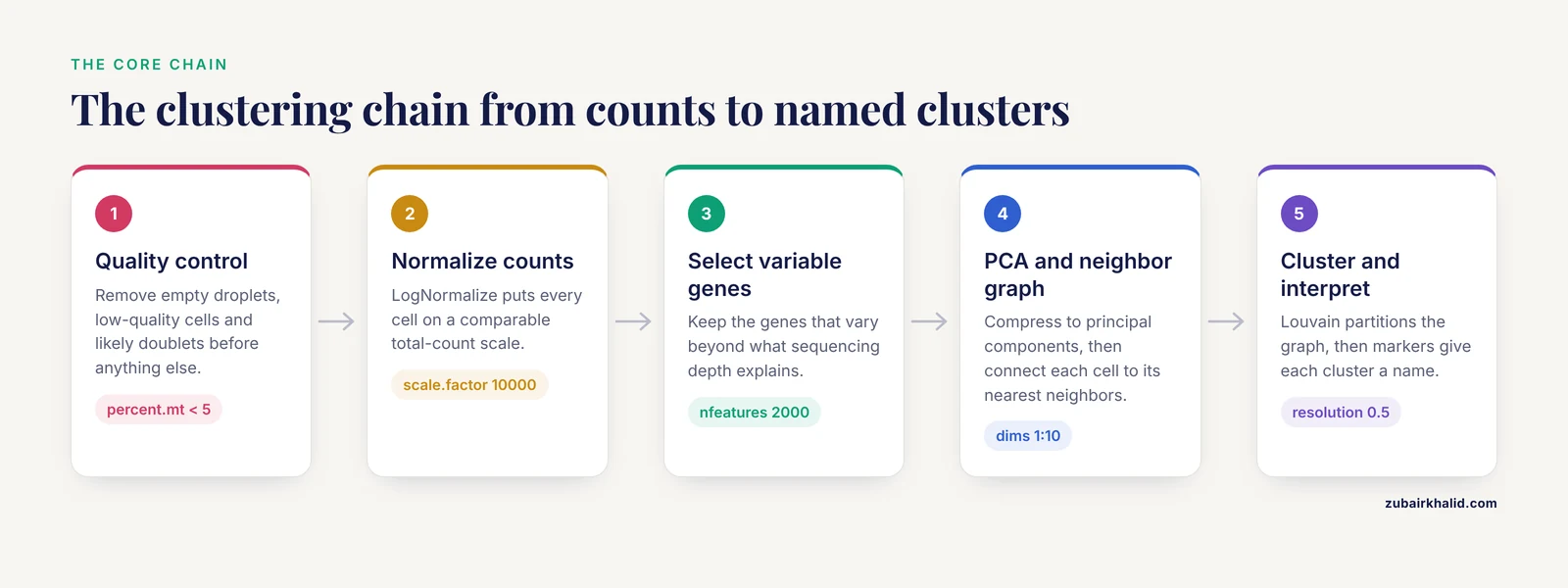
Single-cell clustering is not a single algorithm. It is a chain of decisions, and each link in the chain has parameters that shape the final result:

1. Quality control (QC) removes low-quality cells, empty droplets, and likely doublets so that technical artifacts do not get clustered as biology.
2. Normalization puts each cell on a comparable total-count scale so that differences in sequencing depth do not look like cell types.
3. Feature selection keeps the genes that actually vary between cells, because the 20,000-plus genes in a human genome are mostly noise for clustering purposes.
4. Linear dimensionality reduction (PCA) compresses thousands of variable genes into a few dozen principal components that capture the dominant axes of variation.
5. Graph construction connects each cell to its nearest neighbors in the PCA space. Seurat builds a shared nearest neighbor (SNN) graph, which weights pairs of cells by how many neighbors they share.
6. Community detection partitions that graph into modules. Seurat's FindClusters() runs the Louvain algorithm (or Leiden, if you opt in), which finds groups of cells that are more connected to each other than to the rest of the graph.
7. Interpretation asks which genes define each cluster and what those genes mean biologically.

The reason for PCA before clustering is practical. Cells are described by tens of thousands of gene dimensions, most of which are dominated by technical noise. Euclidean distances in that space are meaningless. Projecting onto the top principal components denoises the space so that nearest-neighbor relationships reflect real transcriptional similarity. Graph-based clustering then handles the fact that single-cell data form continuous manifolds rather than well-separated balls, and it scales to hundreds of thousands of cells, which is why it became the default in Seurat and in most published pipelines [1].

A point worth internalizing early: clustering methods disagree. A benchmark across 12 datasets found that different mainstream methods, including Seurat, produced different numbers of clusters and different assignments on the same data, which is precisely why ensemble approaches that combine several methods were developed [5]. Your job is not to find the one true clustering. It is to choose defensible parameters, check that clusters are stable, and validate them with markers.

Step-by-Step: Clustering the PBMC 3k Dataset

The following walkthrough uses the standard PBMC 3,000-cell dataset. Every step prints its output so you can compare against your own screen.

Step 1. Load the count matrix

Point Read10X() at the directory that contains matrix.mtx.gz, barcodes.tsv.gz, and features.tsv.gz:

pbmc.data <- Read10X(data.dir = "filtered_gene_bc_matrices/hg19/")

pbmc <- CreateSeuratObject(
    counts = pbmc.data,
    project = "pbmc3k",
    min.cells = 3,
    min.features = 200
)
pbmc

Expected output:

An object of class Seurat 
13714 features across 2700 samples within 1 assay 
Active assay: RNA (13714 features, 0 variable features)
 1 layer present: counts

Two arguments filter at load time. min.cells = 3 discards genes detected in fewer than three cells. min.features = 200 discards cells that express fewer than 200 genes, an early and cheap quality screen. In Seurat 5, counts sits in a layer rather than a slot, so code written for Seurat 4 that references pbmc@assays$RNA@counts needs updating to pbmc[["RNA"]]$counts or, better, to accessor functions.

Inspect a few genes if you want reassurance that the data loaded correctly:

pbmc.data[c("CD3D", "CD8A", "MS4A1"), 1:10]

You will see a sparse matrix where most entries are dots. Dots mean zero, not missing data. scRNA-seq count matrices are extremely sparse, typically well over 90 percent zeros in droplet data, which is why they are stored compressed.

Step 2. Quality control

Three metrics form the standard QC trio for every droplet-based dataset [1]:

• nFeature_RNA: the number of genes detected per cell. Low values suggest empty droplets or lysed cells. High values suggest doublets, meaning two cells captured in one droplet.
• nCount_RNA: total UMI counts per cell, where a UMI (unique molecular identifier) is a short barcode attached to each transcript molecule so that duplicates from PCR amplification can be collapsed.
• percent.mt: the fraction of reads mapping to mitochondrial genes. Damaged cells leak cytoplasmic RNA and retain mitochondria, so a high mitochondrial fraction flags poor-quality cells.

Compute the mitochondrial fraction and inspect the distributions:

pbmc[["percent.mt"]] <- PercentageFeatureSet(pbmc, pattern = "^MT-")

VlnPlot(pbmc, features = c("nFeature_RNA", "nCount_RNA", "percent.mt"), ncol = 3)

The pattern = "^MT-" argument matches human mitochondrial gene symbols, which all begin with MT-. For mouse data use "^mt-" (lowercase). For other organisms, check the gene naming convention in your reference annotation before running this line. Getting this pattern wrong is a silent failure. A wrong pattern returns a column of zeros without any warning.

The classic PBMC filtering thresholds from the Seurat workflow are cells with 200 to 2,500 detected genes and mitochondrial percentage below 5 percent:

pbmc <- subset(pbmc, subset = nFeature_RNA > 200 & nFeature_RNA < 2500 & percent.mt < 5)

Look at your violin plots before you apply these numbers blindly. A dataset with stressed or dissociated cells may legitimately need a more permissive mitochondrial cutoff. Tissue type matters too. Single-nucleus datasets, for example, carry higher ambient mitochondrial content than fresh-cell preparations, and their QC thresholds must be set accordingly.

Step 3. Normalize the counts

pbmc <- NormalizeData(pbmc, normalization.method = "LogNormalize", scale.factor = 10000)

LogNormalize divides each cell's gene counts by that cell's total counts, multiplies by 10,000, and natural-log transforms the result. The scale factor 10,000 is a convention that makes values comparable across datasets. The result is stored in a new layer called data.

Seurat also offers SCTransform(), a regularized negative binomial normalization that models the mean-variance relationship per gene. It often produces cleaner clusters on datasets with strong technical variation, but it changes several downstream defaults. The log-normalization route shown here remains the most common in published pipelines and in step-by-step guides [1], so it is the right default while you are learning.

Step 4. Identify highly variable genes

pbmc <- FindVariableFeatures(pbmc, selection.method = "vst", nfeatures = 2000)

top10 <- head(VariableFeatures(pbmc), 10)
top10

Expected output is a character vector of genes like:

 [5] "PPBP" "LYZ"  "S100A9" "IGLL5" "GNLY" "FTL" 
 [7] "PF4"  "FTH1" "CLC"  "MT-CO2"

The vst method models gene variance as a function of mean expression and selects genes that deviate most from that trend, meaning genes that are variable beyond what sequencing depth can explain. Two thousand features is the standard default and works well for datasets in the thousands to low tens of thousands of cells. You do not need to rerun this with different values unless you have a specific reason. Clustering on the full gene set is almost always worse, because the most abundant housekeeping genes dominate the distance calculations.

Step 5. Scale the data

pbmc <- ScaleData(pbmc, vars.to.regress = "percent.mt")

ScaleData centers and scales each gene so that highly expressed genes do not dominate PCA. Regressing out percent.mt removes the mitochondrial signal from the scaled expression matrix. Regression is optional. On a healthy dataset it makes little difference. On a dataset with stressed cells it can remove a technical axis that otherwise contaminates the clusters.

A common tip in single cell clustering Seurat tutorial discussions: ScaleData without arguments scales only the 2,000 variable features, which is what you want. Scaling all 13,714 genes costs memory and adds nothing to clustering.

Step 6. Run PCA and choose the number of dimensions

pbmc <- RunPCA(pbmc, features = VariableFeatures(object = pbmc))

ElbowPlot(pbmc)

ElbowPlot plots the standard deviation explained by each principal component. You pick the number of components at the point where the curve flattens. For PBMC 3k the elbow sits around 10, and the canonical tutorial uses 10 dims throughout. For larger or more heterogeneous datasets the elbow often sits between 30 and 50.

pbmc <- RunPCA(pbmc, npcs = 50)

VizDimLoadings(pbmc, dims = 1:2, reduction = "pca")
DimPlot(pbmc, reduction = "pca")

VizDimLoadings shows which genes drive each component. The first PC in PBMC data is dominated by mitochondrial and ribosomal genes plus immune markers, which is normal. If your first PC is dominated entirely by MT- genes even after regression, your QC cutoffs were too permissive and you should revisit Step 2.

There is also a statistical test, JackStraw, which permutes the data and asks which PCs carry more variance than chance:

pbmc <- JackStraw(pbmc, num.replicate = 100)
pbmc <- ScoreJackStraw(pbmc, dims = 1:20)
JackStrawPlot(pbmc, dims = 1:15)

In practice, the elbow plot plus biological judgment is what most analysts use, because JackStraw is slow on large data and tends to approve more PCs than the elbow suggests.

Step 7. Build the neighbor graph

pbmc <- FindNeighbors(pbmc, dims = 1:10)

Expected output:

Computing nearest neighbor graph
Computing SNN

Two things happened. Seurat found the k nearest neighbors for every cell in the 10-dimensional PCA space, then built the shared nearest neighbor graph on top of them. The dims = 1:10 argument is the single most consequential choice so far. Include too few PCs and you cluster on a denoised but coarse representation, which merges real populations. Include too many and you feed technical noise back in, which shreds populations into fragments.

The second parameter, k.param, defaults to 30 neighbors and rarely needs changing for datasets up to tens of thousands of cells.

Step 8. Cluster the cells

pbmc <- FindClusters(pbmc, resolution = 0.5)

head(Idents(pbmc))

Expected output:

Modularity Optimizer version 1.3.0 by Jeroen Janssens
1. Computing initial partitioning.
2. Adding one node.
3. Restarting from initial partitioning.
...
Modularity Optimizer: 4 iterations
Modularity: 0.8237 in 9 clusters
...

AAACATACAACCAC-1 AAACATTGAGCTAC-1 AAACATTGATCAGC-1 
               1                3                3 
Levels: '0' '1' '2' '3' '4' '5' '6' '7' '8'

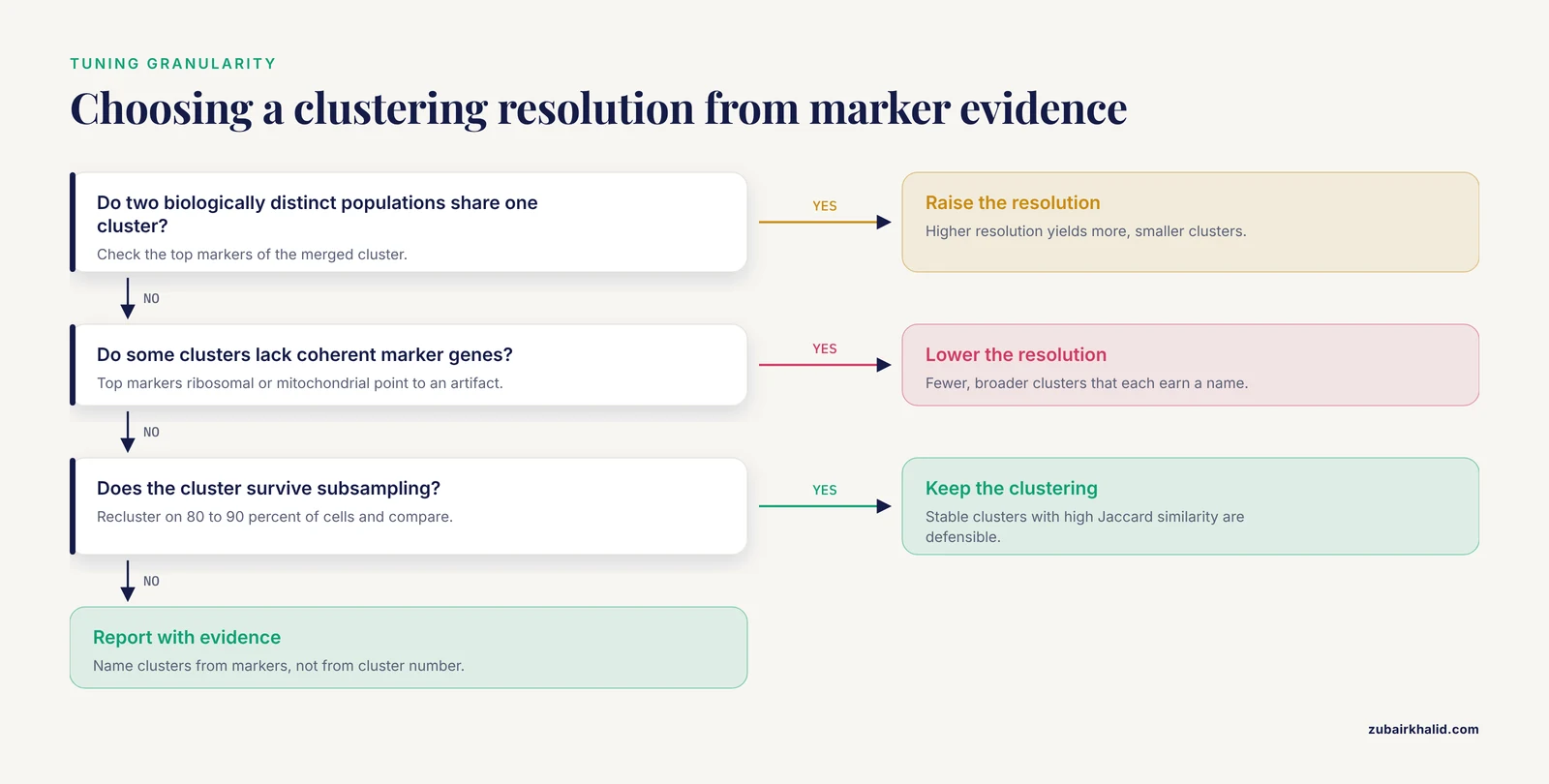
FindClusters runs the Louvain modularity optimization on the SNN graph. The resolution parameter controls how fine the partitioning is. Higher resolution yields more, smaller clusters. Lower resolution yields fewer, broader clusters. Resolution 0.4 to 1.2 covers the useful range for most exploratory analyses, and 0.5 is a reasonable starting point that gives roughly 9 clusters on PBMC 3k, matching the canonical T cell, B cell, monocyte, NK, and dendritic cell composition of that sample.

The cluster identities are stored as the active Idents of the object. Anything you plot by cell identity now uses this clustering. You can change resolution and recluster at any time without repeating PCA:

pbmc <- FindClusters(pbmc, resolution = 1.0)

Seurat keeps the newest result. If you want to compare resolutions, store the identities in metadata first:

pbmc$cluster_r0.5 <- Idents(pbmc)
pbmc <- FindClusters(pbmc, resolution = 1.0)
pbmc$cluster_r1.0 <- Idents(pbmc)

Step 9. Visualize with UMAP

pbmc <- RunUMAP(pbmc, dims = 1:10)
DimPlot(pbmc, reduction = "umap", label = TRUE) + NoLegend()

UMAP (uniform manifold approximation and projection) places cells in two dimensions such that transcriptionally similar cells sit close together. It runs on the same PCA space you clustered on, so dims = 1:10 must match what you used in FindNeighbors. If they disagree, your UMAP and your clusters will not line up, which is a disorienting bug that looks like a biology problem.

UMAP requires the Python package umap-learn. If it is missing you will see an error pointing to the umap-learn package not being available. Install it into the Python environment Seurat is using:

reticulate::py_install("umap-learn")

Two reading rules for UMAP plots. First, distances between clusters are not meaningful. Cluster 0 being far from cluster 3 on the plot does not mean those cell types are more different than two clusters plotted close together. Second, cluster sizes on the plot are shaped by the algorithm's local density preservation and should not be read as cell proportions. Report proportions from the metadata, never from eyeballing the UMAP.

Step 10. Find marker genes

all.markers <- FindAllMarkers(pbmc, only.pos = TRUE,
                              min.pct = 0.25,
                              logfc.threshold = 0.25)

all.markers %>%
    group_by(cluster) %>%
    top_n(n = 5, wt = avg_log2FC)

Expected output structure:

       p_val avg_log2FC pct.1 pct.2 p_val_adj cluster gene
1 4.10e-229   3.14     0.992 0.212        0       0  LTB
2 1.51e-186   2.69     0.943 0.426        0       0  IL7R
...

FindAllMarkers compares each cluster against all other cells and returns genes enriched in each. The parameters filter aggressively:

• only.pos = TRUE keeps genes upregulated in the cluster, which is what you want for annotation
• min.pct = 0.25 requires the gene to be detected in at least 25 percent of cells in either group, which removes genes driven by a handful of cells
• logfc.threshold = 0.25 requires a minimum log2 fold change, which speeds the test by prefiltering

The columns pct.1 and pct.2 show the fraction of cells expressing the gene inside and outside the cluster. A gene with a strong fold change but low pct.1 is expressed in a subpopulation of the cluster, not the whole cluster. Both numbers matter when you pick markers to validate.

Once you see markers such as CD3D and IL7R in one cluster, MS4A1 and CD79A in another, LYZ and S100A9 in a third, you can begin assigning names. A scored dot plot of canonical markers is the fastest survey:

markers <- c("CD3D", "IL7R", "CD8A", "MS4A1", "CD79A",
             "LYZ", "S100A8", "GNLY", "NKG7", "FCER1A", "PPBP")
DotPlot(pbmc, features = markers) + RotatedAxis()

Cluster annotation is a formal discipline with its own pitfalls, particularly when cell types can occupy multiple activation states that share markers, as is the case for dendritic cell subsets where marker panels must distinguish cell type from activation state deliberately [8]. Name clusters from marker evidence, not from cluster number.

Choosing Parameters: A Working Reference

The table below collects the parameters that actually change your result, with their defaults and the situations that call for adjustment.

None of these has a universally correct value, and that is not a flaw in Seurat. Published benchmarking shows that mainstream clustering methods, given the same data, produce materially different numbers of clusters and assignments, with deviations that motivated ensemble methods combining SC3, CIDR, Seurat, and t-SNE plus k-means into a single consensus [5]. Model-based alternatives exist too. DIMM-SC explicitly models UMI counts from droplet data with a Dirichlet mixture model and was benchmarked against Seurat, an example of the broader family of approaches you can turn to when graph-based results feel unstable [9]. Practical consensus in the field: pick parameters from the data (elbow plot, marker biology), not from habit, and validate the result rather than trusting any single run.

Checking That Your Clusters Are Real

Three checks separate a defensible clustering from a pretty picture.

Marker coherence. Each cluster should have a handful of genes with high pct.1, low pct.2, and a biological story. A cluster whose top markers are ribosomal or mitochondrial genes is usually a QC artifact, not a cell type.

Stability under subsampling. Robust clusters survive when you remove cells and recluster. The scclustEval package formalizes this: it subsamples cells, repeats the Seurat clustering, and computes the Jaccard similarity index between cluster assignments across runs. The authors built it precisely because popular algorithms produce different solutions with small changes in the number of PCs, the k-nearest-neighbor parameter, or resolution [10]. In practice, you subsample 80 to 90 percent of cells, recluster at the same parameters, and map clusters between runs. Clusters with high mean Jaccard similarity across resamples are stable. Clusters that dissolve are candidates for merging or for tighter parameters. The package ships with a full Snakemake workflow so the repeated runs are scripted rather than manual [10].

Concordance with independent methods. If a cluster only appears under one algorithm at one parameter setting, treat it as provisional. Ensemble frameworks that pool results from multiple clustering algorithms exist for exactly this reason, and they report both better cluster-number accuracy and better assignments than any single embedded method in their benchmarks [5]. You do not need to run an ensemble for routine work, but when a borderline cluster will drive a paper claim, cross-checking it with a second method such as SC3, a model-based approach like DIMM-SC, or even simple k-means on the PCA embedding is cheap insurance [9].

Common Mistakes and Limitations

Clustering on raw counts. PCA on unnormalized counts is dominated by total UMI counts per cell and by the most highly expressed genes. Clusters then track sequencing depth instead of biology. Always normalize before ScaleData and RunPCA. Symptoms include a UMAP shaped like a smooth gradient of nCount_RNA rather than distinct islands.

Fixing resolution before looking at markers. Analysts often pick resolution 0.8, run once, and name whatever comes out. The correct loop is to cluster at two or three resolutions, check marker coherence at each, and pick the granularity where every cluster earns a name. Changing resolution is cheap. Defending an unjustified cluster list in review is not.

Reading UMAP geometry as truth. UMAP preserves local neighborhoods, not global distances. Two clusters that appear adjacent or adjacent-plus-overlapping may be transcriptionally distant. Use the graph itself and the marker results for claims about relationships between clusters, and use UMAP only as a display layer.

Confusing cluster identity with cell type. A cluster is a group of cells with similar transcriptomes under your parameters. Cell type is a biological claim that requires marker evidence, ideally orthogonal validation. Dendritic cell analysis illustrates the trap clearly, since activation states within one cell type can look transcriptionally distinct enough to separate into clusters that only careful marker-based annotation can resolve correctly [8].

Ignoring doublets. Two cells captured in one droplet form hybrid clusters that look like a coherent population. Cells with very high gene counts and a marker profile spanning two lineages are the usual signature. Droplet-based platforms capture doublets at a low but nonzero rate, and hybrid clusters are most dangerous when they sit between real populations on the UMAP.

Over-filtering QC. Aggressive mitochondrial and gene-count cutoffs can remove genuinely stressed but biologically relevant cells, such as dying tumor cells or activated immune cells with high metabolic demand. Set thresholds from your own violin plots and from knowledge of your tissue, not from a borrowed number. This applies doubly to single-nucleus data, where QC behavior differs from intact-cell preparations [6].

Using mismatched dims across steps. If FindNeighbors used dims = 1:10 and RunUMAP used dims = 1:20, the plot and the clustering describe different spaces. Seurat will not warn you. Check pbmc@reductions$umap@key and, more practically, just confirm the dims arguments match in your script.

Forgetting batch effects across samples. Merging multiple samples without integration clusters cells by sample identity, because technical batch variation between libraries can exceed biological variation between cell types. Seurat's integration workflow ( SplitObject, then IntegrateLayers in Seurat 5) addresses this, and it belongs in the pipeline before FindNeighbors whenever more than one library is present. Integration has its own failure modes and should be run after per-sample QC, not as a substitute for it.

Trusting a single pipeline run. Parameter sensitivity is a documented property of the method, not a user error [10]. Build the stability check into your workflow from the start rather than after a reviewer asks.

What Comes After Clustering

Once clusters are stable and annotated, the standard downstream moves are well served by the same ecosystem.

Differential expression across conditions. For comparisons across subjects or conditions, aggregate cells into pseudobulk counts per cluster per sample and fit a proper statistical model rather than treating individual cells as independent replicates. The dreamlet package implements this with precision-weighted linear mixed models and was shown to handle datasets at the scale of 1.4 million nuclei across hundreds of subjects efficiently [7]. Treating thousands of cells as independent replicates is the single most common statistical error in single-cell differential expression, and pseudobulk aggregation is the standard correction.

Functional interpretation. The SeuratExtend package extends Seurat with integrated functional enrichment, gene regulatory network reconstruction, trajectory inference, and curated visualization, which shortens the path from a cluster of unknown meaning to a testable biological statement [11].

Nucleus-based datasets. If your experiment is single-nucleus rather than single-cell, the same Seurat commands apply with adjusted QC, as documented in tissue-specific workflows such as the skeletal muscle snRNA-seq pipeline built on the 10x Chromium platform [6].

Data exchange. If your collaborators work in Python or your data arrive as AnnData, plan the conversion carefully. A benchmark of conversion tools across 68 datasets found substantial reliability gaps, especially converting H5AD files into R objects, with type changes and failures that appear even below 74,000 cells, so verify feature counts, metadata columns, and a few known gene values after any conversion [3].

Larger public data. When you outgrow toy datasets, standardized repositories built from the Sequence Read Archive offer processed single-cell data at scale, which lets you practice the clustering loop on data with rich known biology [4].

Frequently Asked Questions

How many principal components should I use for clustering?

Use the elbow plot. Pick the PC number where the explained variance curve flattens, typically around 10 for clean PBMC data and 30 to 50 for heterogeneous tissue. Validate by checking whether markers of known cell types separate cleanly at your chosen dimensionality.

What resolution should I choose in FindClusters?

Start at 0.4 to 0.8 and inspect the markers. Raise resolution if two biologically distinct populations are merged, lower it if clusters appear that lack coherent marker genes. There is no universal correct value, so let marker coherence and cluster stability decide.

Why do my clusters change when I change parameters?

Because the clustering is a partition of a graph built from your chosen PCs and neighbors, and small parameter shifts can reassign borderline cells. This is expected behavior of the algorithm, which is why subsampling-based stability checks such as Jaccard similarity analysis exist to distinguish robust clusters from fragile ones.

Do I need to integrate samples before clustering?

Yes, whenever multiple libraries are combined, unless you want clusters that reflect batch rather than biology. Run per-sample QC first, then integrate, then cluster on the integrated embedding. If you have a single library, integration is unnecessary.

Does Seurat 5 change the commands from older tutorials?

Most commands are identical. The main change is that counts and data now live in named layers, and multi-sample integration uses SplitObject and IntegrateLayers instead of the older anchors-only workflow. Code accessing slots directly with @ may need updates.

Can I use this same workflow for single-nucleus RNA-seq data?

Yes, with modified QC. Nuclei have lower total RNA content and different mitochondrial-read behavior than intact cells, so filtering thresholds must be set from your own distributions rather than copied from cell-based tutorials.

How do I know what cell type each cluster is?

Find marker genes with FindAllMarkers, then match the top genes against known canonical markers for your tissue and check expression in a dot plot. Treat annotation as hypothesis testing with marker evidence, and be alert to activation states that can split one cell type into multiple clusters.

Is clustering the same as cell type annotation?

No. Clustering groups cells by transcriptomic similarity under your parameters. Annotation assigns biological identity to those groups using marker genes and reference evidence. A stable cluster with no defensible markers should be reported as an unassigned population rather than given a speculative name.

Sources

1. Single-Cell RNA Sequencing Analysis: A Step-by-Step Overview.
2. A practical guide for single-cell transcriptome data analysis in neuroscience.
3. Benchmarking single-cell format conversion tools reveals interoperability gaps and introduces CrossCell for reliable cross-ecosystem data exchange.
4. scBaseCount: An AI agent-curated, standardized, auto-updated single-cell data repository.
5. SAFE-clustering: Single-cell Aggregated (from Ensemble) clustering for single-cell RNA-seq data.
6. Bioinformatic Workflow for the Analysis of Single-Nucleus RNA-Sequencing Data from Skeletal Muscle.
7. Efficient differential expression analysis of large-scale single-cell transcriptomics data using Dreamlet.
8. Harnessing Single-Cell RNA Sequencing to Identify Dendritic Cell Types, Characterize Their Biological States, and Infer Their Activation Trajectory.
9. DIMM-SC: a Dirichlet mixture model for clustering droplet-based single cell transcriptomic data.
10. Evaluating single-cell cluster stability using the Jaccard similarity index.
11. SeuratExtend: streamlining single-cell RNA-seq analysis through an integrated and intuitive framework.