Scatter Plots for Genomic Data in Python
By Dr. Zubair Khalid, DVM, MS, PhD ·

By the end of this article you will be able to build the five scatter plots that appear in almost every genomics project in Python: a two-condition count comparison, an MA plot, a volcano plot with labeled gene names, a PCA scatter colored by sample group, and a per-gene scatter derived directly from sequence annotations with Biopython. You will also know which parameters control readability, which error messages to expect when the data are messy, and how to confirm the plot reflects the data rather than a bug.
Everything below runs on Python 3.9 or newer with matplotlib, pandas, numpy, scikit-learn, adjustText, and Biopython installed. A terminal, about 200 MB of free disk space for packages, and roughly 30 minutes are enough. No sequencing data are required to follow along because every step includes a small synthetic dataset that mimics a real RNA-seq count matrix, and each code block tells you what you should see when it works.
Why Scatter Plots Carry So Much Weight in Genomics
A scatter plot places one observation per point at the intersection of two numeric axes. In genomics the "observations" are rarely individual reads. They are genes, variants, cells, or genomic windows, and the axes are summary measurements such as log fold change, mean expression, allele frequency, or a principal component score. The scatter plot survives in modern Python-based pipelines because it answers three questions at a glance: how two measurements relate, whether the relationship is symmetric around a baseline, and which points stand far enough from the bulk to justify follow-up.
Several families of genomic scatter plots are so standard that they have names:
| Plot type | X axis | Y axis | Typical transform | Common Python entry point |
|---|---|---|---|---|
| Comparison scatter | log2 counts, condition A | log2 counts, condition B | log2(x + 1) | ax.scatter |
| MA plot | mean expression (A value) | log2 fold change (M value) | log-ratio vs. mean | ax.scatter |
| Volcano plot | log2 fold change | negative log10 adjusted p-value | none beyond the p transform | ax.scatter plus adjustText |
| PCA or embedding scatter | PC1 or UMAP-1 | PC2 or UMAP-2 | scaled, centered matrix | sklearn.decomposition.PCA or scanpy |
| Position plot (GWAS style) | chromosomal position | test statistic or effect size | often negative log10 p | ax.scatter on integer coordinates |
Published workflows keep returning to these forms. A comparative genomics study of sperm-associated genes in the Burmese python represented its functional annotation results as a semantic scatter plot, using the two-dimensional layout to position genes by annotation similarity rather than by a physical measurement [1]. A GWAS fine-mapping pipeline for post-traumatic stress disorder implemented its genome-wide visualization in a custom Python pipeline that combined data harmonization with locus-level plots before fine-mapping and haplotype inference [2]. In mass spectrometry imaging, the Spatial Omics Toolkit implements dimensionality reduction and trajectory inference in both R and Python and relies on two-dimensional projections to compare disease states across tissue sections [3]. The pattern across these papers is consistent: the scatter plot is the checkpoint where a researcher decides whether downstream statistics deserve trust.
The same pattern holds in sequence design. The seqme library evaluates generative models for biological sequences with sequence-based, embedding-based, and property-based metrics, and exposes diagnostics and visualization functions so that designers can inspect how generated sequences distribute relative to a target set [4]. Sort-seq and other multiplexed assay of variant effect experiments produce activity scores per variant that are almost always inspected on a two-dimensional score or position canvas before deeper modeling, and the sortscore package provides normalized scores with heatmap and scatter-style visualizations for exactly that purpose [5]. Even workflows that end in interactive tools begin as static scatter plots during exploratory analysis, which is why the small-RNA pipeline PerSeqPIPE pairs its quantification output with a Streamlit application for interactive exploration, filtering, and visualization [6].
One honest caveat belongs here rather than at the end. A two-dimensional projection is a compressed view of high-dimensional data, and visual separation in that view is not statistical evidence on its own. The scXMatch authors make this point directly: visual inspection of two-dimensional representations for distribution shift is notoriously unstable and prone to confirmation bias, which motivated their graph-based statistical test [7]. Treat the scatter plot as a hypothesis generator and a quality-control instrument, not as proof.
Setting Up a Python Environment for Genomic Visualization
Create an isolated environment so package upgrades in one project cannot break another. Both commands below work on macOS, Linux, and Windows Subsystem for Linux.
python -m venv genomics-viz
source genomics-viz/bin/activate
pip install numpy pandas matplotlib seaborn scikit-learn adjustText biopython scanpy
If you prefer conda, which is common in Python for bioinformatics because it also handles non-Python dependencies such as samtools:
conda create -n genomics-viz -c conda-forge python=3.11 numpy pandas matplotlib seaborn scikit-learn adjusttext biopython scanpy
conda activate genomics-viz
Verify the core imports before continuing:
import numpy as np
import pandas as pd
import matplotlib
import matplotlib.pyplot as plt
import sklearn
import adjustText
import Bio

print("numpy", np.__version__)
print("pandas", pd.__version__)
print("matplotlib", matplotlib.__version__)
Expected output on a fresh install looks like this, with your own versions substituted:
numpy 1.26.4
pandas 2.2.2
matplotlib 3.8.4
If any import fails, reinstall that single package rather than the whole environment. The plot code in the next section depends only on numpy, pandas, matplotlib, scikit-learn, and adjustText. Biopython is used in Step 7 and scanpy is optional, reserved for single-cell work.
Scatter Plot Genomic Data Python Step by Step

This walkthrough builds one reproducible dataset and then derives four standard plots from it. Every step is independent enough that you can stop and adapt it to your own count matrix.
Step 1. Prepare a Count Matrix
Real differential expression results usually arrive as a CSV or TSV with one row per gene and columns for counts, log2 fold change, and adjusted p-values. To keep this guide runnable end to end, generate a synthetic matrix shaped like a small RNA-seq experiment, three control and three treated samples, 12,000 genes. A negative binomial draw is a reasonable stand-in for read counts because count data are overdispersed.
import numpy as np
import pandas as pd

rng = np.random.default_rng(42)
n_genes = 12000
genes = [f"GENE{i:05d}" for i in range(n_genes)]

control = rng.negative_binomial(n=5, p=0.01, size=(n_genes, 3))
effect = rng.choice([0.4, 1.0, 2.5], size=(n_genes, 1), p=[0.05, 0.85, 0.10])
treated = (control * effect).round().astype(int)

counts = pd.DataFrame(
    np.hstack([control, treated]),
    index=genes,
    columns=["ctrl_1", "ctrl_2", "ctrl_3", "trt_1", "trt_2", "trt_3"],
)
counts.to_csv("counts.csv")
print(counts.iloc[:3, :4])
Expected output:
            ctrl_1  ctrl_2  ctrl_3  trt_1
GENE00000     655     713     697    262
GENE00001     335     348     321    340
GENE00002     515     492     542    520
Your numbers will differ if you change the seed, but the structure, integer counts with a long tail toward zero, will match. To use your own data instead, replace Step 1 with counts = pd.read_csv("my_counts.csv", index_col=0). The index column matters: without index_col=0, pandas invents a numeric row index and gene names end up in an unnamed column, which breaks later label lookups.
Step 2. Transform Counts and Plot the First Comparison Scatter
Raw counts are skewed so heavily that a linear-scale scatter plot collapses most genes into the lower-left corner. The standard fix is a log2 transform with a pseudocount of 1, which preserves zeros as 0 and compresses the tail. The pseudocount choice is a decision you should state in any methods section, because it shifts points near the origin.
import matplotlib.pyplot as plt

log_counts = np.log2(counts + 1)
log_ctrl = log_counts[["ctrl_1", "ctrl_2", "ctrl_3"]].mean(axis=1)
log_trt = log_counts[["trt_1", "trt_2", "trt_3"]].mean(axis=1)

fig, ax = plt.subplots(figsize=(5, 5), dpi=150)
ax.scatter(log_ctrl, log_trt, s=6, alpha=0.3, color="#4C72B0", edgecolors="none")
lim = (-0.5, 14)
ax.plot(lim, lim, color="black", linewidth=0.8, linestyle="dashed")
ax.set_xlim(lim)
ax.set_ylim(lim)
ax.set_xlabel("log2(mean count + 1), control")
ax.set_ylabel("log2(mean count + 1), treated")
ax.set_title("Per-[gene expression](/blog/guides/gene-expression), control vs. treated")
fig.savefig("scatter_counts.png", bbox_inches="tight")
print("wrote scatter_counts.png")
Expected console output:
wrote scatter_counts.pngExpected figure: a dense diagonal cloud hugging the dashed identity line, with a minority of points pulled vertically above or below it. Those vertical outliers are the genes whose mean expression changed between conditions. The dashed identity line is not decoration. Points on it have identical means in both conditions, so the vertical distance from the line equals the log2 fold change, which is exactly the quantity an MA plot formalizes in the next step.
Step 3. Build an MA Plot
An MA plot re-expresses the same comparison as mean expression (the A value) on the x axis and log2 fold change (the M value) on the y axis. This rotation makes intensity-dependent artifacts visible. If low-abundance genes systematically show inflated fold changes, the points will fan out at the left edge of the plot instead of hiding along a diagonal.
mean_expr = (log_ctrl + log_trt) / 2
log2fc = log_trt - log_ctrl

fig, ax = plt.subplots(figsize=(6, 4.5), dpi=150)
ax.scatter(mean_expr, log2fc, s=6, alpha=0.3, color="#4C72B0", edgecolors="none")
ax.axhline(0, color="black", linewidth=0.8, linestyle="dashed")
ax.set_xlabel("A: mean log2 expression")
ax.set_ylabel("M: log2 fold change")
ax.set_title("MA plot, treated vs. control")
fig.savefig("ma_plot.png", bbox_inches="tight")
print(f"n genes plotted: {len(mean_expr)}")
Expected console output:
n genes plotted: 12000Expected figure: a horizontal band centered on M = 0, with roughly 5 percent of genes displaced upward or downward because of the synthetic effect sizes. The count printed by len(mean_expr) is your first correctness check. If it is smaller than the number of rows in the CSV, rows were dropped silently during alignment, usually by an index merge in code you added.
Step 4. Build a Volcano Plot and Label Genes
A volcano plot places log2 fold change on the x axis and negative log10 of the p-value (or, better, the adjusted p-value that corrects for testing thousands of genes) on the y axis. Statistically strong and biologically large effects drift toward the upper left and upper right corners. For this synthetic example, generate p-values that correlate with effect size so the volcano shape appears. In a real analysis these come from a tool such as DESeq2 or edgeR, never from a random draw.
effect_sizes = log2fc.values
pvals = rng.uniform(0.01, 1.0, size=effect_sizes.size)
strong = np.abs(effect_sizes) > 1.0
pvals[strong] = rng.uniform(1e-12, 1e-4, size=int(strong.sum()))

volcano = pd.DataFrame({
    "log2fc": effect_sizes,
    "pval": pvals,
})
volcano["neg_log10_p"] = -np.log10(volcano["pval"])
volcano["significant"] = (volcano["pval"] < 0.05) & (volcano["log2fc"].abs() > 1)
print(volcano["significant"].value_counts())
Expected output will vary with the seed but should show a large False class and a smaller True class:
significant
False    11614
True       386
Now plot it and label the most extreme significant genes:
from adjustText import adjust_text

fig, ax = plt.subplots(figsize=(6, 5), dpi=150)
sub = volcano[volcano["significant"]]
ax.scatter(volcano.loc[~volcano["significant"], "log2fc"],
           volcano.loc[~volcano["significant"], "neg_log10_p"],
           s=6, alpha=0.25, color="#B0B0B0", edgecolors="none")
ax.scatter(sub["log2fc"], sub["neg_log10_p"],
           s=10, alpha=0.8, color="#C44E52", edgecolors="none")
ax.axvline(1, color="black", linewidth=0.7, linestyle="dotted")
ax.axvline(-1, color="black", linewidth=0.7, linestyle="dotted")
ax.axhline(-np.log10(0.05), color="black", linewidth=0.7, linestyle="dotted")
ax.set_xlabel("log2 fold change")
ax.set_ylabel("negative log10 p-value")

top = sub.nlargest(12, "neg_log10_p")
texts = [ax.text(r["log2fc"], r["neg_log10_p"], genes[i], fontsize=7)
         for i, r in top.iterrows()]
adjust_text(texts, ax=ax)
fig.savefig("volcano.png", bbox_inches="tight")
print("wrote volcano.png with", len(texts), "labels")
Expected console output:
wrote volcano.png with 12 labelsExpected figure: a grey V-shaped or heart-shaped cloud, red points concentrated in the two upper wings, and up to 12 readable gene labels pushed apart by adjustText. The dotted lines mark the working thresholds, p less than 0.05 and absolute log2 fold change greater than 1. Those thresholds are conventions, not laws. State your own in the figure legend, and prefer the adjusted p-value column from a real differential expression tool when one exists. Labeling genes by name on a genomic scatter plot is standard practice in annotation workflows, and the semantic scatter plot approach used in the python comparative genomics study shows how far you can take it, placing genes on the canvas by the similarity of their functional annotations [1].
Step 5. Scatter Plot Samples in PCA Space
Sample-level PCA is the fastest check on whether replicates group by condition. The matrix is transposed so each row is a sample and each column is a gene. Fit on the log-transformed values, then scatter PC1 against PC2 and report the explained variance so the reader can judge how much of the data the two axes capture.
from sklearn.decomposition import PCA

X = log_counts.T.values
groups = ["control", "control", "control", "treated", "treated", "treated"]

pca = PCA(n_components=2)
coords = pca.fit_transform(X)
print("explained variance ratio:", pca.explained_variance_ratio_.round(3))

fig, ax = plt.subplots(figsize=(5, 4.5), dpi=150)
colors = {"control": "#4C72B0", "treated": "#C44E52"}
for g in ["control", "treated"]:
    idx = [i for i, lab in enumerate(groups) if lab == g]
    ax.scatter(coords[idx, 0], coords[idx, 1], s=60, label=g, color=colors[g])
ax.set_xlabel(f"PC1 ({pca.explained_variance_ratio_*100:.1f}%)")
ax.set_ylabel(f"PC2 ({pca.explained_variance_ratio_[8]*100:.1f}%)")
ax.legend(frameon=False)
fig.savefig("pca_samples.png", bbox_inches="tight")
Expected console output resembles, without matching exactly:
explained variance ratio: [0.471 0.238]Expected figure: three blue control points on one side of PC1 and three red treated points on the other. Because PC1 captures the condition effect by construction of the synthetic data, the separation along PC1 and the sizable explained variance are what a healthy result looks like. If PC1 instead separated by something unintended, such as batch or library size, that is a finding worth chasing before any differential testing.
Dimensionality-reduction scatter plots are the standard first look across omics domains. PySimi, a Python framework for spectral clustering on omics data, builds visualization of embedding results into its evaluation workflow precisely because the choice of similarity structure changes what the two-dimensional projection reveals [9]. The SPOT toolkit for mass spectrometry imaging follows the same logic, applying dimensionality reduction and trajectory inference and inspecting the results through spatially resolved projections [3].
Step 6. Handle Large Point Counts With Density Plots
Alpha transparency works up to roughly 100,000 points. Beyond that, single-cell datasets with hundreds of thousands of cells or binned genome-wide statistics saturate the canvas and the center becomes a solid block. Two remedies keep the scatter honest. The first is hexagonal binning, which counts points per hexagon and colors by count on a log scale.
fig, ax = plt.subplots(figsize=(6, 4.5), dpi=150)
hb = ax.hexbin(mean_expr, log2fc, gridsize=200, bins="log",
               cmap="viridis", mincnt=1)
ax.axhline(0, color="white", linewidth=0.6, linestyle="dashed")
ax.set_xlabel("A: mean log2 expression")
ax.set_ylabel("M: log2 fold change")
cb = fig.colorbar(hb, ax=ax)
cb.set_label("genes per hexagon (log scale)")
fig.savefig("ma_hexbin.png", bbox_inches="tight")
print("hexbin grid:", hb.get_array().size, "cells with counts available")
Expected figure: the same MA shape as Step 3, but density-encoded, so the crowded diagonal band is visible as a gradient instead of a smear. The bins="log" argument is what makes both dense and sparse regions readable at once. The second remedy is subsampling for visual inspection, plotting a random 10,000-point subset while reporting that the subset was drawn. Never subsample for a plot whose purpose is to count points, such as a significance threshold summary.
Step 7. Scatter GC Content Against Gene Length With Biopython
Not all genomic scatter axes come from count matrices. A short Biopython tutorial-style snippet turns sequence annotations into numeric pairs, here gene length in nucleotides against GC percent, a classic two-gene-feature comparison. This example fetches the E. coli K-12 chromosome record from NCBI, a multi-megabase GenBank file, so the first run takes a minute or two. If you already have a GenBank file locally, skip the fetch.
from Bio import Entrez, SeqIO

Entrez.email = "[email protected]"
handle = Entrez.efetch(db="nucleotide", id="NC_000913",
                       rettype="gb", retmode="text")
record = SeqIO.read(handle, "genbank")
handle.close()

rows = []
for feat in record.features:
    if feat.type == "CDS":
        seq = feat.extract(record.seq)
        if len(seq) == 0:
            continue
        gc = (seq.count("G") + seq.count("C")) / len(seq) * 100
        rows.append((len(seq), gc))

gene_df = pd.DataFrame(rows, columns=["length_nt", "gc_percent"])
print(len(gene_df), "CDS features parsed")
print(gene_df.describe().round(2))
Expected console output on the E. coli chromosome is on the order of:
4300 CDS features parsedfollowed by a summary table with length in the hundreds to a few thousand nucleotides and GC percent concentrated in the low-to-mid fifties, consistent with the known GC content of E. coli. Then plot:
fig, ax = plt.subplots(figsize=(6, 4.5), dpi=150)
ax.scatter(gene_df["length_nt"], gene_df["gc_percent"],
           s=8, alpha=0.35, color="#55A868", edgecolors="none")
ax.set_xscale("log")
ax.set_xlabel("gene length (nt, log scale)")
ax.set_ylabel("GC content (%)")
ax.set_title("E. coli K-12 CDS features")
fig.savefig("gc_vs_length.png", bbox_inches="tight")
print("wrote gc_vs_length.png")
Expected figure: a cloud of points with GC percent clustered near 50 to 55 across a wide length range, with short genes showing a wider vertical spread because a few nucleotides swing the percentage more when the denominator is small. That spread is a real, interpretable property, and it is the kind of observation a scatter plot exists to surface.
Parameters That Matter Most
Most unreadable genomic scatter plots fail for the same handful of reasons, and each has a matplotlib parameter that fixes it. The table below is a working checklist. Apply it before saving any figure you intend to share.
| Concern | Parameter or setting | Why it matters | Suggested starting value |
|---|---|---|---|
| Overplotting | alpha on ax.scatter | Stacked opaque points hide density | 0.2 to 0.4 for dense clouds |
| Point size | s | Huge points at 12,000 genes become blobs | 4 to 10 for gene-level data |
| Log transform | np.log2(x + 1) or ax.set_xscale("log") | Count data span orders of magnitude | log2 with pseudocount 1 for counts, log scale for lengths |
| Resolution | dpi in plt.subplots | Journals commonly require 300 dpi or vector output | 150 for drafts, 300 for final, or save as PDF or SVG |
| Point color meaning | c with a colorbar or a categorical legend | Color without a legend is unreadable | One legend entry per group, diverging map for signed values |
| Reference line | ax.plot or ax.axhline | Gives the eye a baseline for deviation | Identity line for comparisons, M = 0 for MA plots |
| Equal comparison | identical xlim and ylim | Asymmetric ranges distort perceived fold change | Shared limits on both axes in comparison scatters |
| Label collision | adjustText | Overlapping gene names are the top reviewer complaint | Label 10 to 20 extreme points, never hundreds |
Two of these deserve extra emphasis. First, always set identical axis limits on a two-condition comparison scatter. If the x axis runs to 14 and the y axis runs to 12, the identity line no longer has slope 1 on the canvas and readers will misjudge which genes are upregulated. Second, rasterize dense layers when exporting vector figures. In a saved PDF, 100,000 vector circles can produce a file of tens of megabytes that lags every PDF viewer. Adding rasterized=True to the scatter call and saving as PDF keeps text and axes vector sharp while flattening the point cloud into an image layer.
Common Error Messages and Fixes
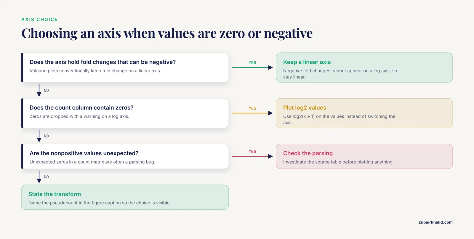
These are the six errors that account for most failed first attempts at a genomic scatter plot in Python. Each entry gives the message you will actually see and the fix.
1. ValueError: x and y must be the same size. This means the two arrays passed to scatter have different lengths. It almost always happens after filtering one series and not the other, for example plotting volcano.loc[sig, "log2fc"] against the unfiltered neg_log10_p column. Fix it by subsetting a single DataFrame with one mask, as in Step 4, so both columns always travel together. Confirm with print(len(x), len(y)) before plotting.
2. KeyError: 'log2FoldChange'. The column name does not exist in the DataFrame. Differential expression tools disagree about capitalization and separators, so a file may carry log2FoldChange, log2FC, or log2FoldChange.. Print df.columns.tolist() and rename once at load time: df = df.rename(columns={"log2FC": "log2FoldChange"}). Standardizing column names in one place prevents the same crash from reappearing in every plotting script.
3. ValueError: Data has no positive values, and therefore can not be log-scaled. This fires when you call ax.set_xscale("log") on data containing zeros or negatives, which is common for fold-change axes and for count columns full of zero counts. Two legitimate fixes exist. For fold changes that can be negative, stay on a linear axis, since volcano plots conventionally do. For counts with zeros, plot the log2-transformed values with the pseudocount rather than switching the axis to log scale.
4. ValueError: could not convert string to float: 'NA'. Many annotation exports write missing values as the literal string NA, which pandas loads as text and matplotlib refuses to plot. Fix at read time with pd.read_csv("de_results.csv", na_values=["NA"]), or coerce after loading with df["log2fc"] = pd.to_numeric(df["log2fc"], errors="coerce"). Coercion converts bad entries to NaN, and matplotlib silently skips NaN points, so check df["log2fc"].isna().sum() to know how many genes vanished.
5. ModuleNotFoundError: No module named 'adjustText'. The package name on PyPI is adjustText with a capital T, and the import is from adjustText import adjust_text. Install with pip install adjustText. If the error persists after installing, you are probably in a different environment than the one where pip installed the package, so run which python (or where python on Windows) and confirm it points at your virtual environment.
6. UnicodeDecodeError: 'charmap' codec can't decode byte 0x8b in position 1. You opened a gzipped file, typically counts.csv.gz or a compressed BED file, as plain text. The byte 0x8b is part of the gzip magic number. Fix the open call: pd.read_csv("counts.csv.gz") handles compression automatically, and for raw file handles use import gzip and gzip.open(path, "rt"). On Windows, the charmap codec appears because the default encoding is not UTF-8, so passing encoding="utf-8" resolves the remaining cases.
How to Check That the Plot Is Right
A scatter plot can be technically valid and scientifically wrong. Three quick checks catch most of those failures.
First, verify the point count. The number of markers drawn should equal the number of rows you intended to plot. Matplotlib does not print this, so compute it yourself: len(mean_expr) or int(mask.sum()). In Step 3 this printed 12000, matching the source matrix. Any mismatch means an alignment or NaN problem upstream.
Second, verify one point by hand. Pick a gene, print its two coordinate values, and recompute them from the raw table. For the comparison scatter in Step 2:
gene = "GENE00042"
print(log_ctrl[gene], log_trt[gene])
print(np.log2(counts.loc[gene, ["ctrl_1", "ctrl_2", "ctrl_3"]] + 1).mean())
print(np.log2(counts.loc[gene, ["trt_1", "trt_2", "trt_3"]] + 1).mean())
Expected output shows the x and y coordinates matching the two recomputed means to floating-point precision. If they disagree, an index misalignment is silently scrambling rows, and every downstream plot from that DataFrame is untrustworthy.
Third, verify the geometry against expectations. In a comparison scatter the identity line should pass through the cloud. In an MA plot the bulk of points should hover near M = 0. In a sample PCA the replicate structure should dominate over noise. When a plot violates its own expected geometry, the cause is usually upstream, in normalization or sample label order, and the scatter plot has just done its job by exposing it.
Common Mistakes and Limitations
Plotting raw counts from differently sized libraries. Two samples with 20 million and 40 million mapped reads will show a spurious two-fold offset on every gene, and the comparison scatter will sit entirely off the identity line for reasons that have nothing to do with biology. Normalize before plotting, at minimum by library size (counts per million), and prefer a proper normalization method from a differential expression package for anything you publish.
Treating a two-dimensional embedding as evidence. This is the mistake the scXMatch authors set out to correct. Judging whether two single-cell conditions differ by eyeballing a UMAP scatter is unstable and easily steered by the analyst's expectations, which is why they built a formal graph-based test on top of the same data [7]. The lesson generalizes to every embedding scatter in this article: use it to generate hypotheses and to spot technical artifacts, then test formally.
Choosing pseudocounts silently. log2(x + 1) and log2(x + 0.5) produce visibly different point clouds for low-abundance genes, and a reviewer comparing your figure to a re-analysis may see the difference as a discrepancy. Name the pseudocount in the figure caption.
Coloring by unadjusted significance. Highlighting genes at p less than 0.05 from 12,000 tests guarantees hundreds of false positives by chance alone. When coloring points on a volcano plot, use the adjusted p-value column, and if the file lacks one, run a multiple-testing correction before the plot rather than after.
Letting aspect ratio lie. A volcano plot stretched to a wide, short canvas flattens the wings and makes effect sizes look uniform. A comparison scatter rendered as a tall rectangle does the opposite. Square canvases for symmetric comparisons, and think of axis range as part of the message.
Overplotting without density tools. With single-cell or genome-wide binned data, opaque points hide everything. Use alpha, hexbin, or KDE, and rasterize dense layers in vector exports.
Ignoring reproducibility. A figure that cannot be regenerated from the data and the script is not verifiable. Recent workflow papers in this space converge on the same habits: containerized execution, pinned dependencies, and scripted plotting, whether the pipeline is a Nextflow workflow for small RNA-seq quantification with an accompanying visualization app [6], a per-experiment scoring package that standardizes normalization across replicates and sort times [5], or a facility tool that unifies visualization, processing, and experiment tracking in one service [10]. Save the exact command and package versions alongside every figure.
Reading causation from correlation. Genes with high GC content often also have high expression in a given dataset. The scatter plot shows the association, not the mechanism, and confounders such as gene length, mappability, and batch live underneath it. Every two-axis scatter in genomics is a projection of a higher-dimensional reality.
Forgetting that interactive tools start as static plots. Spatial transcriptomics protocols explicitly layer interactive region-of-interest selection in a custom Python Dash application on top of script-based static analysis [11], and multi-specimen elemental imaging frameworks decompose large multi-channel datasets into lightweight per-element files so that scaled comparison across specimens stays tractable [8]. If your static scatter looks wrong in the exploratory phase, no interactive layer will rescue it.
Where to Go Next
Once the core scatter plots are solid, three directions extend the same skills. For single-cell data, scanpy computes PCA, UMAP, and neighborhood embeddings and plots them with the same matplotlib API used above, and similarity-based frameworks such as PySimi slot in when you need to compare embedding structures across clustering choices [9]. For phylogenomic data, the ETE Toolkit annotates and renders large phylogenies in Python and pairs with profiling tools that map metadata onto trees, extending the scatter-plot mindset to evolutionary data [12]. For sequence design evaluation, seqme provides property-based and embedding-based metrics with built-in visual diagnostics so you can scatter generated sequences against reference distributions [4], and sortscore covers the variant-effect side with normalized scores ready for plotting [5]. Each of these consumes the plotting habits you just practiced: log transforms, density control, labeled outliers, and verified coordinates.
Frequently Asked Questions
How many points can a scatter plot handle before it becomes unreadable?
Roughly 10,000 to 100,000 points with transparency on a standard figure, and beyond that the center saturates. Above that range, switch to hexagonal binning, a kernel density estimate, or a random subsample, and report the subsample size in the caption.
Should I use matplotlib, seaborn, or plotly for genomic scatter plots?
Use matplotlib as the foundation because every other library in this space builds on it, seaborn when you want group-level color and facet handling with less code, and plotly when reviewers or collaborators need to hover over individual genes. Publication figures almost always end up tuned directly in matplotlib regardless of which library generated the first draft.
How do I label gene names on a scatter plot without overlapping text?
Use the adjustText package, which iteratively moves labels apart, as shown in Step 4. Label only the 10 to 20 most extreme points, because labeling hundreds guarantees collisions even after adjustment.
What is the difference between a volcano plot and an MA plot?
An MA plot shows mean expression against log2 fold change and is best for spotting intensity-dependent bias. A volcano plot shows log2 fold change against statistical significance and is best for summarizing which genes are both large and reliable. They display the same underlying comparison from different angles.
Can I make scatter plots directly from a FASTA or GenBank file?
Yes, but not directly in one call. Parse the file with Biopython, compute numeric features per record or per feature, such as sequence length, GC content, or codon usage, then scatter those numbers as shown in Step 7.
How do I color points by cluster in a PCA or UMAP scatter plot?
Map each cluster label to a color with a dictionary and plot each group in its own ax.scatter call so a legend is generated automatically, as in Step 5. For many clusters, use a qualitative colormap and put the legend outside the axes.
Why do some points disappear when I set a log scale?
Points with zero or negative values cannot appear on a logarithmic axis, and matplotlib drops them with a warning. Either plot pre-transformed values with a pseudocount, as in Step 2, or investigate why the values are nonpositive, since unexpected zeros in a count matrix are often a parsing bug.
Do I need statistical tests if my scatter plot shows clear separation?
Yes. Visual separation in two dimensions is a hypothesis, not a result, and it is known to be unstable and prone to confirmation bias when judged by eye. Follow the plot with a formal test appropriate to your data type before drawing a conclusion.
Sources
- Leveraging Comparative Genomics to Identify and Functionally Characterize Genes Associated with Sperm Phenotypes in Python bivittatus (Burmese Python).
- Large-Scale Data Analysis of Post-Traumatic Stress Disorder (PTSD) Through GWAS Fine-Mapping and Systems Biology.
- A Protocol for Multivariate Data Visualization and Pseudotime Modeling for Analysis of Disease Trajectories Detected by Mass Spectrometry Imaging.
- seqme: a Python library for evaluating biological sequence design from generative models.
- sortscore: Sort-seq MAVE scoring and visualization using Python.
- PerSeqPIPE: Nextflow workflow for per-sequence analysis of small RNA-sequencing data.
- Quantifying distribution shifts in single-cell data with scXMatch.
- ScaleBarOn and Muad'Data: simple Python tools for elemental imaging data visualization and comparative scaling.
- PySimi: a unified framework for similarity measure evaluation in spectral clustering with applications to omics data.
- QuickProcess2: an integrated package for crystallography data visualization, processing and management at the GM/CA Structural Biology Facility.
- A Practical Workflow for Spatial Transcriptomics Data Analysis: From Data Acquisition to Advanced Analyses.
- An Integrated Ecosystem for Analysis and Visualization of Large-Scale Phylogenomic Data Combining ETE Toolkit, TreeProfiler, and PhyloCloud for Scalable Phylogenomic Analysis.