How to Validate and Test Your RNA-seq Workflow
By Dr. Zubair Khalid, DVM, MS, PhD ·

By the end of this guide you will be able to turn an RNA-seq pipeline into a tested, versioned project that fails loudly when something breaks, run its tests automatically on every commit, validate each layer from read quality through differential expression with reference data and known-answer checks, and choose between Nextflow and Snakemake on concrete criteria instead of habit.
Have the following installed or available before you start:
- A machine or hosted CI runner with at least 2 CPUs and 8 GB RAM for smoke tests (full runs need more)
- Nextflow (Java 17 or newer) or Snakemake 8 (Python 3.11 or newer)
- conda or mamba, and optionally Docker or Apptainer
- FastQC, fastp, STAR (or HISAT2), featureCounts, and MultiQC
- R 4.x with edgeR and limma installed from Bioconductor
- seqkit, for downsampling test data
- Git, plus a GitHub or GitLab repository with hosted runners
- One representative FASTQ pair and a STAR genome index for your organism
RNA-seq workflow testing and CI/CD validation matter because every processing stage shapes the final gene list. Read alignment, transcript quantification, normalization, and the statistical method used to call differentially expressed genes each influence the accuracy and sensitivity of the analysis, and each stage can add false positives or false negatives [1]. A pipeline that exits with status zero can still drift for weeks before anyone notices. The walkthrough below makes that drift visible and automatic.
Why RNA-seq Workflows Drift and Why Testing Catches It
RNA-seq pipelines fail in three ways, and each needs a different kind of test.
- Crashes. A tool exits nonzero, a file is missing, the run stops. These are loud, and a plain exit-code check catches them.
- Silent metric drift. The run completes, but uniquely mapped reads slide from 92 percent to 78 percent after a tool update, or duplication creeps up after a kit lot change. Quiet, and caught only by metric gates.
- Statistical drift. The run completes, the metrics look fine, and the differentially expressed gene list changes anyway because a default changed upstream. Quietest of all, and caught only by comparing outputs against a frozen reference.
Drift has predictable sources: dependency updates, reference genome patches, new annotation releases, and changed software defaults. Cross-study comparisons suffer when reference genomes and tool versions are inconsistent across analyses, and a standardized reanalysis platform for fungal pathogens restored near-perfect correlation with published results even across annotation version differences [2]. Testing converts each drift source into a signal. Unit assertions catch crashes, metric gates catch silent drift, and frozen-reference comparisons catch statistical drift.
Choosing a Bioinformatics Workflow Manager: Nextflow vs Snakemake
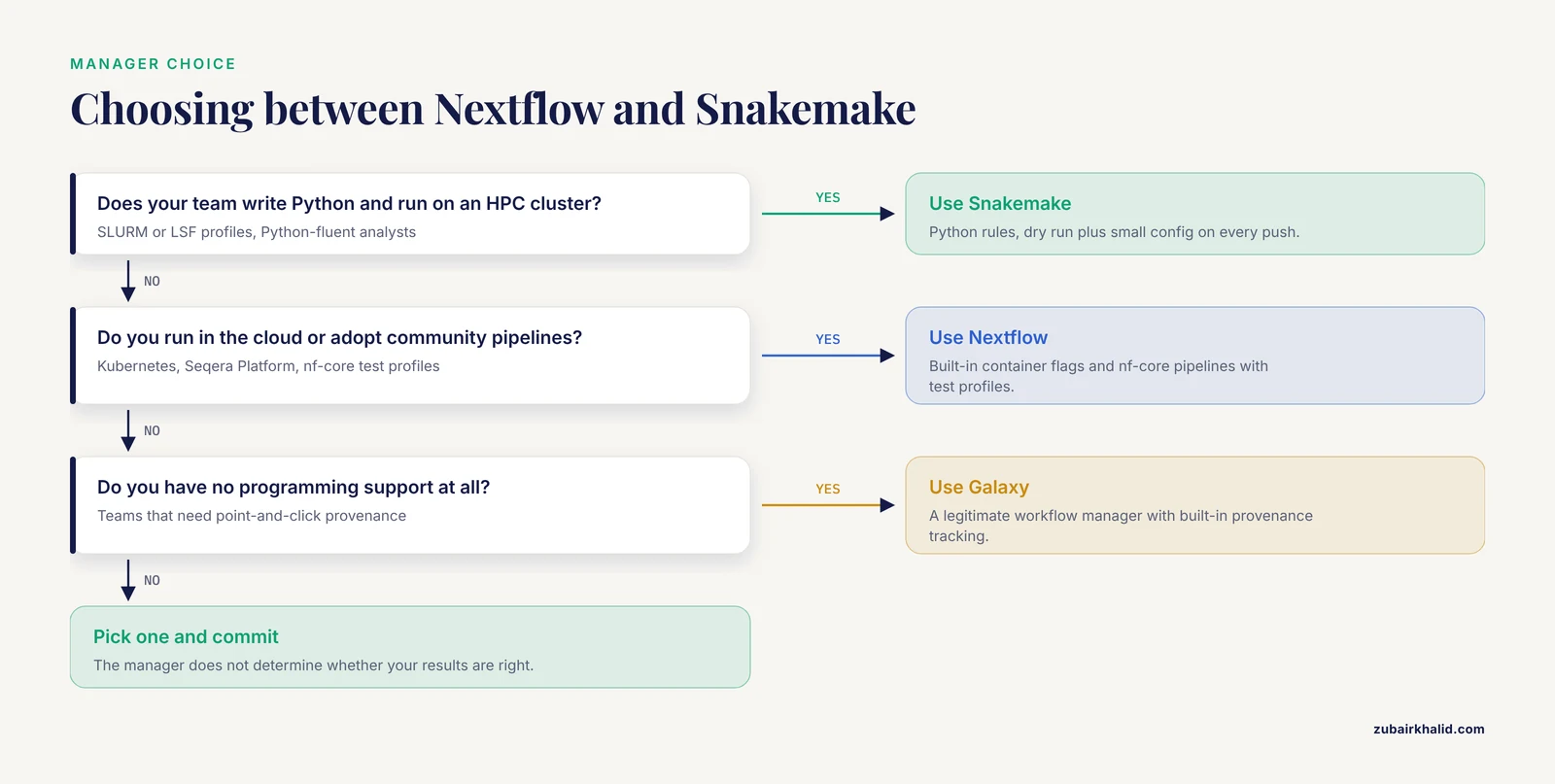
A bioinformatics workflow manager is software that chains tools into a directed graph of steps, tracks inputs and outputs, skips finished work on reruns, and records per-step metadata such as versions and command lines. If you are still running RNA-seq analyses as a folder of one-off shell scripts, adopting a manager is the single highest-value change you can make, because every test and CI feature below depends on it.
Nextflow and Snakemake are the two managers most widely used for RNA-seq. Both are mature, and both appear in demanding settings. IntegrateALL, a clinical-grade pipeline that standardizes B-ALL RNA-seq analysis from FASTQ all the way to rule-based subtype assignment across 26 WHO-HAEM5/ICC entities, is built on Snakemake [3]. On the Nextflow side, the nf-core community collection provides curated RNA-seq pipelines that ship with test data and CI configuration you can copy into your own project.
| Criterion | Nextflow | Snakemake |
|---|---|---|
| Language | Groovy-based DSL | Python |
| Rerun model | Asynchronous dataflow, caches completed processes | DAG rule matching, reruns only changed targets |
| Containers | Built-in -with-docker, -with-singularity, -with-conda | -use-conda, plus container integration |
| Strongest environment | Cloud and Kubernetes, Seqera Platform | HPC clusters (SLURM, LSF profiles) |
| Ecosystem | nf-core curated pipelines with bundled test profiles | Common in methods papers and clinical pipelines |
| Typical CI pattern | nextflow run -profile test on every push | Dry run plus small config on every push |
Practical decision rules:
- If your team writes Python and your compute lives on an HPC cluster, Snakemake will feel natural.
- If you run in the cloud, or you want to adopt community pipelines wholesale instead of writing your own, Nextflow has the advantage.
- Point-and-click platforms such as Galaxy are also legitimate workflow managers with built-in provenance tracking, and they suit teams without programming support.
- The worst option is no manager at all. Scripts cannot be tested, resumed, or pinned reliably.
Pick one, commit to it for the project, and move on to validation. The manager does not determine whether your results are right.
The Three Layers of RNA-seq Workflow Validation
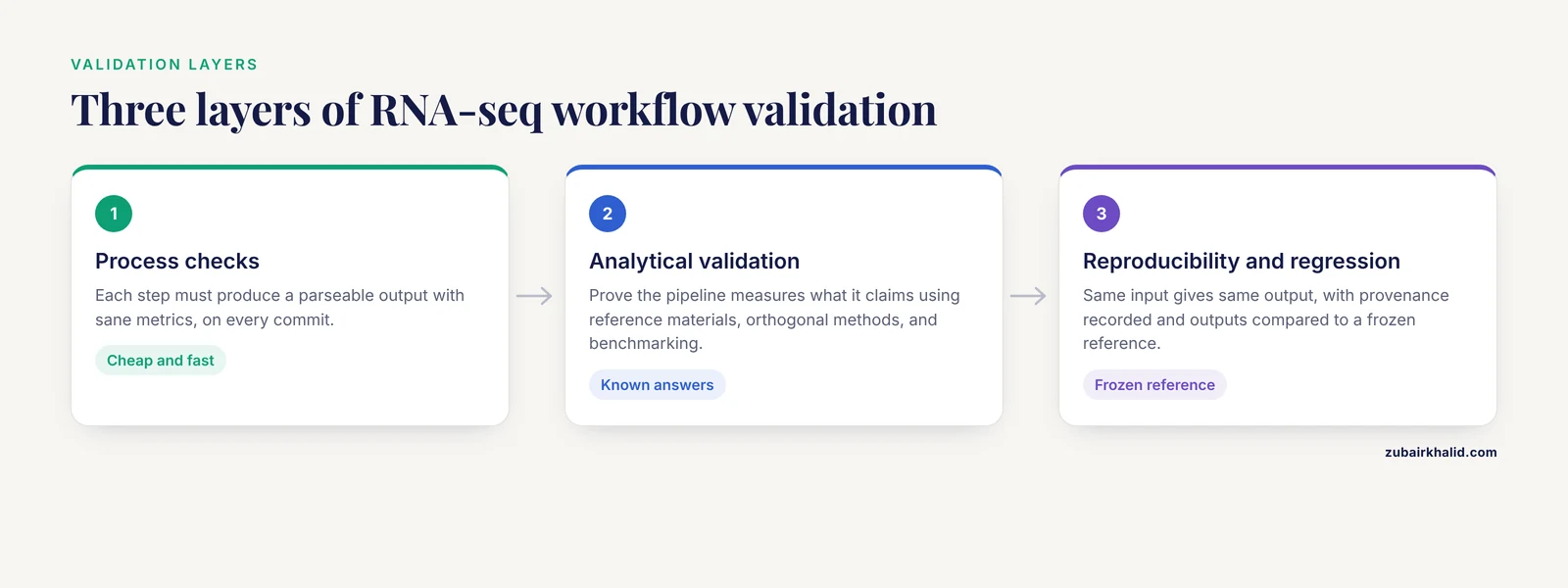
Layer 1: Process Checks
Every step must produce a parseable output with sane metrics. FastQC produces a report, STAR produces a Log.final.out that parses, featureCounts produces a count matrix with the expected number of columns. These checks answer "did each step run and produce something reasonable." They are cheap, fast, and belong in every commit.
Layer 2: Analytical Validation
Analytical validation answers a harder question: does the pipeline measure what it claims to measure? Three established patterns exist.
First, reference materials. A clinical laboratory validating a targeted RNA-seq panel for hematologic malignancies ran it against a reference DNA (NA12878), a commercial reference RNA, 14 normal peripheral blood samples, and bone marrow samples with known gene fusions, then on 30 clinical samples across seven malignancy categories [4]. The pattern generalizes to any RNA-seq pipeline: include at least one sample with a known, expected answer.
Second, orthogonal methods. A platelet RNA biomarker study for non-small-cell lung cancer measured ITGA2B by RNA-seq, then by qPCR in a test cohort (AUC 0.922, 95% CI 0.892 to 0.952, sensitivity 92.8%, specificity 78.6%) and an independent validation cohort (AUC 0.888, sensitivity 91.2%, specificity 56.5%), and confirmed the signal again with droplet digital PCR (AUC 0.967) [5]. The design pattern matters more than the numbers: a test cohort, an independent validation cohort, and an orthogonal platform.
Third, benchmarking against alternative tools, covered in its own section below.
Layer 3: Reproducibility and Regression
The same input must give the same output this month and next month. That requires provenance: tool versions, genome build, annotation release, and command lines recorded with every run. Work on standardized pathogen analysis addressed this by forcing AI assistants to invoke Galaxy's native tools rather than manipulating data directly, so provenance stayed intact, and by providing standalone notebooks for anything outside the platform [2]. Independent reproduction is the strongest form of this layer. One undergraduate course recreated a clinical recurrence-risk workflow from a single breast cancer patient library split across twelve barcoded sequencing preparations, and reproduced the key molecular subtype and biomarker calls with standard QC and quantification tools.
RNA-seq Workflow Testing and CI/CD Validation, Step by Step
Continuous integration (CI) means an automated runner executes your tests on every commit. Continuous delivery (CD) means a passing commit is packaged as a versioned, runnable release. For an RNA-seq pipeline this translates into a fast smoke test on each push and a scheduled full regression against frozen references.
Step 1: Pin Every Version
Unpinned software is the root of most silent drift. Pin with conda environment files or containers. One environment file per tool keeps solves fast and failures readable.
# envs/star.yaml
name: star
channels:
  - conda-forge
  - bioconda
dependencies:
  - star = 2.7.10b
  - samtools = 1.19.2
conda env create -f envs/star.yaml
conda run -n star star --versionExpected output:
2.7.10bIf you prefer containers, build your own image once, push it to your registry, and freeze the tag in the pipeline configuration. Never reference a moving tag such as latest.
// nextflow.config (excerpt)
params.genome_build        = "GRCh38"
params.annotation_release  = "GENCODE v44"

process {
    withName: 'STAR_ALIGN' {
        container = 'registry.example.com/rna-seq/star:2.7.10b'
    }
}
Whenever a pinned version changes, treat it as a schema change: rerun everything downstream and refresh the frozen reference outputs described in Step 9.
Step 2: Build a Small, Fixed Test Dataset
Your test data must be small enough to run in minutes and fixed so that every run sees identical bytes. Downsample one representative sample pair to roughly 1 percent of its reads.
conda create -n pipeline-tools -c conda-forge -c bioconda \
    seqkit fastqc fastp multiqc -y

seqkit sample -p 0.01 -s 42 sample_R1.fastq.gz -o test_R1.fastq.gz
seqkit sample -p 0.01 -s 42 sample_R2.fastq.gz -o test_R2.fastq.gz

seqkit stats test_R1.fastq.gz test_R2.fastq.gz
Expected output (your numbers will differ):
file              format  type  num_seqs    sum_len    min_len  avg_len  max_len
test_R1.fastq.gz  FASTQ   DNA   213,842     32,076,300 150      150      150
test_R2.fastq.gz  FASTQ   DNA   213,842     32,076,300 150      150      150
Parameter notes:
-p 0.01keeps about 1 percent of reads.-s 42fixes the random seed so the same reads are kept every time.- Using the same seed on both mates keeps pairs synchronized, which the equal
num_seqsvalues above confirm.
Commit the test FASTQ files to the repository (Git LFS works well) or commit a small download script keyed to a public run accession. Four samples, two control and two treated, are enough for a smoke test that exercises the whole pipeline including the statistics layer.
Step 3: Encode the Pipeline With a Test Profile
Give the pipeline a dedicated test profile so CI and humans run the identical thing.
// nextflow.config (excerpt)
profiles {
    test {
        params.input      = 'assets/test_samples.csv'
        params.outdir     = 'results/test'
        params.max_cpus   = 2
        params.max_memory = '4 GB'
    }
}
sample,fastq_1,fastq_2
ctrl_1,test_R1.fastq.gz,test_R2.fastq.gz
ctrl_2,test_R1.fastq.gz,test_R2.fastq.gz
treat_1,test_R1.fastq.gz,test_R2.fastq.gz
treat_2,test_R1.fastq.gz,test_R2.fastq.gzFor Snakemake, the equivalent is a config/test.yaml with the same sample table, and a dry run to inspect the plan before executing:
snakemake -n --cores 2 --configfile config/test.yamlExpected output ends with the job list and the line This was a dry-run. The -n flag plans without executing, which makes it a fast structural test on its own.
Step 4: Add Per-Step Assertions
Assertions turn quiet drift into loud failures. The most useful single assertion for bulk RNA-seq is a mapping-rate gate parsed straight from the STAR logs.
#!/usr/bin/env bash
# bin/check_mapping_rate.sh
set -euo pipefail

LOG_DIR="${1:?usage: check_mapping_rate.sh <log_dir> <floor>}"
FLOOR="${2:?usage: check_mapping_rate.sh <log_dir> <floor>}"

shopt -s nullglob
logs=("$LOG_DIR"/*/Log.final.out)
if (( ${#logs[@]} == 0 )); then
    echo "FAIL: no STAR logs found under $LOG_DIR"
    exit 1
fi

for log in "${logs[@]}"; do
    pct=$(awk -F'|' '/Uniquely mapped reads %/ {gsub(/ +/, "", $2); print $2}' "$log")
    sample=$(basename "$(dirname "$log")")
    if awk -v a="$pct" -v b="$FLOOR" 'BEGIN { exit ((a+0) < (b+0)) ? 0 : 1 }'; then
        echo "FAIL: $sample uniquely mapped ${pct}% (floor ${FLOOR}%)"
        exit 1
    fi
    echo "PASS: $sample uniquely mapped ${pct}%"
done
bash bin/check_mapping_rate.sh results/test/star 80.0Expected output:
PASS: ctrl_1 uniquely mapped 91.4%
PASS: ctrl_2 uniquely mapped 90.8%
PASS: treat_1 uniquely mapped 88.2%
PASS: treat_2 uniquely mapped 89.6%
How to choose the floor: derive it from your own baseline, not from a paper. If your last 50 full runs show uniquely mapped reads between 84 and 95 percent, a floor of 80 flags real problems without nagging on every run. Add the same pattern for other gates: test -s on output files catches empty outputs, and a row-count check on the count matrix catches silent annotation failures.
Step 5: Aggregate QC With MultiQC
multiqc results/test -o results/test/multiqcExpected output ends with:
Analysis complete for 8 samplesMultiQC parses FastQC, STAR, featureCounts, and Salmon outputs into one report and one machine-readable table under multiqc_data/. In CI, upload the report as an artifact so a failing build still shows you why it failed:
- uses: actions/upload-artifact@v4
  if: always()
  with:
    name: multiqc-report
    path: results/test/multiqc/
Step 6: Add a Statistics Smoke Test
The differential expression layer deserves its own test, because the standard Bioconductor flow of importing counts, filtering low-expression genes, normalizing, and fitting a model is where many silent failures live [6]. A smoke test proves the layer runs end to end on real counts and retains a plausible number of genes.
# bin/de_smoke_test.R
library(edgeR)

counts  <- read.delim("results/test/counts/genes.count_matrix.tsv", row.names = 1)
targets <- read.csv("assets/test_samples.csv")
group   <- factor(sub("_[0-9]+$", "", targets$sample))

y <- DGEList(counts = counts, group = group)
keep <- filterByExpr(y, group = group)
y <- y[keep, , keep.lib.sizes = FALSE]
y <- calcNormFactors(y, method = "TMM")

cat("Genes retained after filtering:", nrow(y), "\n")
stopifnot(nrow(y) > 1000)
Expected output:
Genes retained after filtering: 12487Parameter notes: filterByExpr drops genes too lowly expressed to support a useful test, calcNormFactors with the default TMM method corrects composition bias, and the stopifnot line converts a suspicious result (for example, 30 retained genes after an annotation mismatch) into a build failure.
A worked normalization example makes the units concrete. A gene with 1,200 raw counts in a library of 3.2 million mapped reads has a counts-per-million value of 1,200 divided by 3.2, which equals 375 CPM. If a downstream step reports that gene at 0.375, a thousand-fold unit error is hiding somewhere, and the smoke test is where you want to find it.
Step 7: Add a Known-Answer Test
Smoke tests prove the statistics layer runs. Known-answer tests prove it is right. ERCC spike-in mixes carry known concentration ratios between mix 1 and mix 2, so a correct pipeline recovers the expected direction of change for the large majority of spike-in transcripts.
# after fitting mix2 vs mix1 with glmQLFit and glmQLFTest
spike_ids <- grep("^ERCC-", rownames(fit$coefficients), value = TRUE)
expected  <- sign(read.csv("assets/ercc_expected_sign.csv")$sign)
observed  <- sign(fit$table$logFC[spike_ids])

frac_correct <- mean(observed == expected)
cat("Spike-ins with expected direction:", round(frac_correct, 3), "\n")
stopifnot(frac_correct >= 0.80)
If you lack spike-ins, substitute a public positive-control dataset with a strong, well-characterized perturbation and assert the expected direction for a pre-specified gene set. The clinical panel literature shows the same logic at higher rigor, where a new assay is run against samples with known fusions and reference RNA before it touches patient material [4].
Step 8: Wire Up CI
GitHub Actions is the most common hosted option. The workflow below runs the smoke test on every push and on pull requests, and schedules a nightly run with the same profile so external changes (base image updates, runner changes) get caught too.
# .github/workflows/pipeline-tests.yml
name: rna-seq-pipeline-tests
on:
  push:
    branches: [main]
  pull_request:
  schedule:
    - cron: "0 3 * * *"   # nightly at 03:00 UTC

jobs:
  smoke-test:
    runs-on: ubuntu-latest
    steps:
      - uses: actions/checkout@v4
      - uses: actions/setup-java@v4
        with:
          distribution: temurin
          java-version: "17"
      - name: [Install Nextflow](/knowledge/bioinformatics/install-nextflow)
        run: curl -s https://get.nextflow.io | bash
      - name: Run test profile
        run: ./nextflow run main.nf -profile test -ansi-log false
      - name: Assert outputs
        run: |
          test -s results/test/multiqc/multiqc_report.html
          bash bin/check_mapping_rate.sh results/test/star 80.0
          Rscript bin/de_smoke_test.R
      - uses: actions/upload-artifact@v4
        if: always()
        with:
          name: multiqc-report
          path: results/test/multiqc/
The Snakemake equivalent replaces the Nextflow steps with:
      - uses: actions/setup-python@v5
        with:
          python-version: "3.12"
      - run: pip install "snakemake>=8"
      - run: snakemake --cores 2 --use-conda --configfile config/test.yaml
Parameter notes: -cores 2 caps concurrency to the runner's size, -use-conda materializes the pinned environments from Step 1, and the cron expression 0 3 * means 03:00 UTC daily. A green build means the pipeline ran, every assertion passed, and the statistics layer retained a plausible gene set. That is the minimum bar for merging a change.
Step 9: Add Regression Checks Against a Frozen Reference
At each release, freeze the count matrix and the MultiQC metrics table into the repository or the release assets. Every subsequent run compares against them. This is the only test that catches statistical drift.
# bin/regression_check.R
new <- read.delim("results/test/counts/genes.count_matrix.tsv", row.names = 1)
ref <- read.delim("test/reference/counts_reference.tsv", row.names = 1)

sample_id <- "ctrl_1"
stopifnot(sample_id %in% names(new), sample_id %in% names(ref))

r <- cor(new[[sample_id]], ref[[sample_id]], method = "spearman")
if (r < 0.995) {
  stop(sprintf("Regression failed: Spearman r = %.4f (floor 0.995)", r))
}
cat("Regression passed: Spearman r =", sprintf("%.4f", r), "\n")
Expected output:
Regression passed: Spearman r = 0.9999When this check fails, diff versions first: the tool version, the genome build, the annotation release, and any changed default. A small Spearman drop with identical versions usually points at a changed reference file rather than a changed tool. Refresh the frozen reference deliberately, in a reviewed commit, never silently.
Step 10: Record Provenance and Tag Releases
Capture a run report and trace with every run so any result can be traced to exact versions and commands.
./nextflow run main.nf -profile test \
    -with-report report.html -with-trace trace.txt

snakemake --cores 2 --use-conda --report report.html
Then tag validated states so collaborators can name exactly what they ran:
git tag -a v1.3.0 -m "Validated against reference set 2026-06"
git push origin v1.3.0
The frozen reference outputs from Step 9 belong to the tag. A release is then a self-describing package: code, pinned environments, test data, reference outputs, and the reports that prove the validation ran.
Common Errors During Testing and Their Exact Fixes
Process `FASTQC` terminated with an error exit status (1)Nextflow prints the work directory above this message. Read .command.err inside it. Usual causes: a wrong FASTQ path in the samplesheet, a tool missing from the pinned image, or an out-of-memory kill. Fix the cause, not the symptom, and rerun.
MissingInputException in line 12 of /path/Snakefile
Missing input files for rule star_align: test_R1.fastq.gz
Snakemake resolves inputs relative to the working directory. Run from the repository root or correct the paths in config/test.yaml.
EXITING because of FATAL error: genome index mismatchSTAR builds its index for a specific read length, 100 by default. Reads of a different length need an index regenerated with the matching read length. Rebuild the index and update the pinned reference in the same commit.
PackagesNotFoundError: The following packages are not available from current channels:
  - star=9.9.9
A typo in a pinned version. Check what exists with conda search -c bioconda star and pin a real version.
Error in file(file, "rt"): cannot open the connectionThe R smoke test ran before the pipeline produced its outputs, or the outdir path changed. In CI, order the steps so assertions run after the pipeline step, and fail fast on the first missing file.
Process completed with exit code 1In CI this is your assertion script talking. Read the FAIL: line above it before rerunning anything.
What Good Looks Like: Metrics, Formulas, and Acceptance Gates
| Check | Formula or source | What a failure usually means |
|---|---|---|
| Uniquely mapped percent | STAR Log.final.out, field "Uniquely mapped reads %" | Wrong index, contamination, or degraded RNA |
| Duplication percent | FastQC or Picard metrics | Overamplification or very low input |
| rRNA fraction | Counts against an rRNA annotation | Failed rRNA depletion |
| CPM | Raw counts divided by library size in millions | Missing or wrong normalization step |
| TMM factor | edgeR calcNormFactors on filtered counts | Composition bias between groups |
| BH-adjusted FDR | p multiplied by m over rank, capped at 1 | Unadjusted p values leaking into reports |
| Replicate Spearman r | cor(counts_A, counts_B) across genes | Label swap or batch failure |
| PCA grouping | First two PCs of the top variable genes | Batch effects larger than the treatment |
Two habits make these gates trustworthy. First, derive thresholds from your own historical distribution (for example, flag anything below your 5th percentile) rather than copying a number from another tissue, protocol, or lab. Second, keep the gates in version control next to the pipeline, so a threshold change is a reviewed, dated decision.
Testing the Statistics Layer
The standard Bioconductor pattern is worth restating because it defines what your statistics test must cover: import and organize counts, filter and normalize, then model with a negative binomial or voom linear model with empirical Bayes moderation, followed by gene set testing [6]. Interactive tools such as Glimma let reviewers examine individual samples and genes during that review.
Workflow choices inside that pattern change the answer. Alignment, quantification, normalization, and the statistical method each influence which genes are called differentially expressed, including the false positives and false negatives, which is why the statistics layer needs its own validation rather than inheriting trust from the plumbing [1]. Packaged analysis systems make this layer inspectable: iDEP connects 63 R and Bioconductor packages across a large set of species and lets users download the exact R code behind each analysis, which is precisely the property you want in a validated statistics layer [7].
Honest handling of null results is part of statistics-layer validation. A reanalysis of public COPD lung tissue data reported a null finding for SFTPD (log2 fold change 0.316, FDR 0.421) together with an effect size (Cohen's d = 0.42) and a post-hoc power estimate of 23 percent, then checked the transcriptomic conclusion against an independent microarray cohort (GSE47460) [8]. Effect sizes and power statements belong in your validation reports, not just p values.
Validating RNA-seq Based Models and Classifiers
If your workflow ends in a classifier rather than a gene list, validation design dominates everything else. A reanalysis of single-cell RNA-seq data combining mutation-derived and expression features showed run-level repeated stratified cross-validation reaching balanced accuracy 0.973 (SD 0.113), while grouping validation by donor proxy (leave-one-GSM-out) dropped it to 0.708, and permutation testing at the group level was not significant (p = 0.257) [9]. The lesson is structural: put all data from one biological unit in the same fold, and keep preprocessing inside each fold so it cannot leak.
External validation is the second requirement. A COVID-19 severity model trained on cohorts from Berlin and Bonn and tested on completely unseen cohorts from Stanford and Korean medical centers held an AUROC of 1.0 in Korea and 0.86 (CI 0.81 to 0.9) in Stanford, which is what robustness across hospitals looks like when it exists [10]. A narrative review of bulk RNA-seq machine learning in oncology frames the full path from preprocessing through model validation, including deconvolution as a lower-cost alternative to single-cell composition estimates, and is a useful checklist for designing your own model validation [11].
Normalization is the third requirement for low-input material. Liquid biopsy RNA-seq work that integrated multiple feature types through an ensemble classifier also benchmarked intra-sample normalization methods and evaluated performance across ten datasets with independent test sets, precisely because poor biomarker reproducibility often traces back to normalization and validation gaps [12].
Benchmarking Your Pipeline Against Alternatives
Run a second tool on the same input and compare outputs before you trust either one. DoTT-ML, a condition-aware pipeline for detecting transcriptional readthrough, was benchmarked against ARTDeco and DoGFinder across three public datasets (influenza A virus total RNA-seq, HSV-1 nascent 4sU-RNA, and HSV-1 Z-RNA RIP-seq) using ROC AUC comparisons, and its key biological call, a stable readthrough transcript at the Scd1 locus under dietary stress in mouse liver, was confirmed experimentally [13]. That two-step pattern, computational benchmark plus orthogonal confirmation, is the template for validating any novel analysis step.
Full pipelines can be validated the same way. IntegrateALL was evaluated on 615 independent test samples (accuracy 0.98, F1-score 0.96), applied to 774 unselected B-ALL cases with unambiguous subtype assignment in 81.5 percent, and reproduced across three independent cohorts totaling 436 samples [3]. You do not need that scale for an internal pipeline, but you should copy the structure: a held-out test set, an unselected application, and at least one external cohort.
Annotation assumptions deserve the same scrutiny as tools. In small RNA-seq work on an incompletely annotated species, adding orthologue information increased the number of confidently annotated miRNAs, while cross-mapping against other non-coding RNAs prevented false miRNA calls [14]. If your organism is poorly annotated, validate the annotation the way you validate software.
A practical benchmarking recipe: fix the input bytes, run tool A and tool B with pinned versions, compare outputs with correlation and a discordance rate, then manually inspect the top discordances before deciding which tool to standardize on.
Common Mistakes and Limitations
- Confusing "ran without errors" with "produced correct results." A pipeline can be perfectly reproducible and consistently wrong. Each layer needs its own evidence, which is why the three layers exist.
- Unpinned dependencies. Moving tags and unpinned conda solves change under you. Freeze versions, and treat any version bump as a reason to refresh frozen references.
- Reference and annotation drift. Changing the genome build or annotation release invalidates counts downstream. Re-run everything affected, record the release, and update the regression references in the same change.
- Over-downsampling test data. At very low depth, QC metrics become unstable and the test stops representing the real run. Confirm that test metrics track your full runs before trusting the gates.
- Copying thresholds from other labs. Tissue, protocol, and library type shift every distribution. Derive gates from your own baseline.
- Leakage in model validation. Splitting at the run level when samples share a donor inflates accuracy dramatically. Group folds by biological unit and keep preprocessing inside folds.
- Validating on one sample or one gene. A single qPCR check is a sanity check, not a validation. Use a test cohort, an independent cohort, and an orthogonal platform for anything that matters.
- Reporting p values without effect sizes or power. Null results especially need power statements and external checks to be interpretable.
- Testing only the happy path. Inject failures deliberately: corrupt a FASTQ, point at a missing reference, swap two sample labels. The pipeline should fail loudly, not produce a plausible-looking report.
- Skipping scheduled runs. A pipeline tested only at release time drifts between releases. Nightly regression catches dependency and runner changes that arrive from outside your repository.
- Confusing reproducibility with correctness. Identical outputs across runs prove determinism, not validity. Layer 2 evidence is separate and mandatory.
On limitations: validation demonstrates that a workflow behaves as specified on the data you tested, and it does not replace biological interpretation. Individual analyses, especially diagnostic or clinical ones, need review by a qualified bioinformatician or molecular pathologist before any decision is based on them.
Frequently Asked Questions
What does CI/CD mean for an RNA-seq workflow?
Continuous integration means a runner executes your pipeline tests automatically on every commit, and continuous delivery means a passing commit is packaged as a versioned release. In practice this is a fast smoke test on each push plus a scheduled regression run against frozen reference outputs.
Nextflow vs Snakemake: which bioinformatics workflow manager should I choose?
Choose based on your team and infrastructure, because both are mature and correct results come from validation rather than the manager. Snakemake suits Python-fluent teams on HPC clusters, while Nextflow suits cloud-heavy teams and anyone adopting community pipelines that ship ready-made test profiles.
How large should my RNA-seq test dataset be?
Small enough to finish in minutes and large enough that QC metrics stay stable. A downsampled pair in the low hundreds of thousands of reads per sample is a common starting point, and you should confirm that test metrics track your full runs before trusting the gates.
How do I validate the differential expression layer?
Run it on a positive-control dataset or spike-in mixes where the direction of change is known, assert the expected direction, and keep the code pinned so outputs match a frozen reference. Filtering, normalization, and modeling choices all change the gene list, so test them as a unit.
How often should RNA-seq regression tests run?
Smoke tests on every push, full regression nightly or weekly, and always before a release tag. Scheduled runs catch dependency and reference updates that arrive from outside your repository.
Which metrics should fail a CI build?
Any assertion you define: a missing output file, an empty count matrix, a mapping rate below your baseline-derived floor, or a Spearman correlation against reference counts below your threshold. Derive floors from your own historical runs rather than from another lab's tissue or protocol.
How do I validate an RNA-seq based classifier or biomarker?
Use independent test cohorts, group cross-validation folds by biological unit so all data from one donor stays in one fold, and confirm key calls on an orthogonal platform such as qPCR or ddPCR.
Do I need containers if I already use conda environments?
No, conda environment files with pinned versions are a valid alternative. Containers make CI more deterministic because the same image runs on your laptop, the cluster, and the runner, so use them whenever your CI supports them.
Sources
- RNA-seq assistant: machine learning based methods to identify more transcriptional regulated genes
- Standardizing RNA-seq Analysis of Fungal Pathogens Using BRC-Analytics and Agentic AI: A Candidozyma auris Case Study.
- IntegrateALL: An end-to-end RNA-seq analysis pipeline for multilevel data extraction and interpretable subtype classification in B-precursor ALL
- Diagnostic Validation of a Clinical Laboratory-Oriented Targeted RNA Sequencing System As a Comprehensive Assay for Hematologic Malignancies
- Development and Validation of Tumor-educated Blood Platelets Integrin Alpha 2b (ITGA2B) RNA for Diagnosis and Prognosis of Non-small-cell Lung Cancer through RNA-seq
- RNA-seq analysis is easy as 1-2-3 with limma, Glimma and edgeR
- iDEP: an integrated web application for differential expression and pathway analysis of RNA-Seq data
- Transcriptomic Evaluation of SFTPD Expression in COPD Lung Tissue Using RNA-Seq
- Integrating Mutation-Derived and Expression Features from Single-Cell RNA Sequencing: Pitfalls of Standard Cross-Validation in Small-Cohort Settings
- Robust Machine Learning predicts COVID-19 Disease Severity based on Single-cell RNA-seq from multiple hospitals
- Machine Learning Models for Cancer Research: A Narrative Review of Bulk RNA-Seq Applications
- Assessing the complementary information from an increased number of biologically relevant features in liquid biopsy-derived RNA-Seq data
- DoTT-ML: Condition-aware detection of transcriptional readthrough from RNA-seq with optional ML-based prioritization
- Small RNA-seq analysis of single porcine blastocysts revealed that maternal estradiol-17beta exposure does not affect miRNA isoform (isomiR) expression.