Quantification Strategies in RNA-seq Pipelines
By Dr. Zubair Khalid, DVM, MS, PhD ·

featureCounts counts reads against gene annotations from a BAM file, Salmon estimates transcript abundances directly from reads using quasi-mapping, and RSEM aligns reads to a reference and uses an expectation-maximization model to assign reads to transcripts. The rule of thumb is simple: if your biological question is gene-level differential expression in a well-annotated organism, featureCounts after a splice-aware alignment is the workhorse choice. If you need transcript or isoform resolution, or you want to quantify without aligning to the genome, Salmon or RSEM is the better fit. A 2019 benchmark of lncRNA quantification adds a critical nuance: for long non-coding RNAs, pseudoalignment methods and RSEM outperformed featureCounts and HTSeq at both sample- and gene-level comparisons, and gene-counting methods systematically underestimated lncRNA expression [1].
This article walks through what quantification actually means in an RNA-seq pipeline, explains each of the three tools on its own terms, compares them side by side, gives worked scenarios, and covers how to wire the whole thing into a reproducible workflow with a modern bioinformatics workflow manager.
What Quantification Means in an RNA-seq Pipeline
Quantification is the step that turns millions of sequencing reads into numbers you can analyze. Every read in an RNA-seq experiment comes from a fragment of an RNA molecule. Quantification asks, for each gene or transcript in your annotation, how many fragments support it. Those numbers become the input matrix for differential expression analysis, clustering, biomarker work, or any downstream model.
Three distinct quantities matter, and confusing them is the root of many pipeline mistakes:
- Raw fragment counts. The number of reads or read pairs assigned to a feature. Counts are the input that count-based differential expression tools such as DESeq2 and edgeR expect.
- Estimated transcript abundance. Expression of each transcript isoform, usually reported as TPM (transcripts per million, a relative abundance measure normalized by transcript length) or estimated counts that account for ambiguous assignment.
- Effective length-normalized expression. Because longer transcripts produce more fragments per molecule, methods normalize by the effective length of the transcript after subtracting fragment-size effects.
A further wrinkle: RNA-seq reads are short, many span exon junctions, and transcripts in the same gene family share exons. Some reads cannot be uniquely assigned to a single feature. The quantification strategy you pick is really a strategy for handling that ambiguity, and different tools handle it very differently.
featureCounts, Salmon, and RSEM Options in Detail
These three tools represent the three dominant quantification strategies in bulk RNA-seq pipelines. Each approaches the assignment problem from a different direction.
featureCounts: Alignment-Based Gene Counting
featureCounts, part of the Subread package, takes an aligned BAM file and a gene annotation in GTF or GFF format, then counts how many reads overlap the features you specify. It is an alignment-based gene quantification method, in the same category as HTSeq-count [1].
The core logic is overlap counting. A read is assigned to the gene whose exonic regions it overlaps, subject to rules you set:
- Strandedness. The
-sflag specifies the library orientation. Use-s 1for stranded (sense) libraries,-s 2for reverse-stranded, and-s 0for unstranded. Getting this wrong silently swaps read assignments on antisense transcripts. - Paired-end handling. The
-pflag tells featureCounts to count fragments rather than individual reads, so a read pair contributes one count. - Feature granularity.
-t exon -g gene_idcounts at the gene level by summing exonic overlap per gene. You can count at other levels, for example per exon, by changing these arguments. - Multi-mapping and ambiguous reads. By default, reads that overlap multiple genes are discarded rather than counted. This is the behavior that most affects genes with many overlapping isoforms or paralogous genes.
A typical gene-level count command looks like this:
featureCounts -s 1 -p -t exon -g gene_id \
  -a annotation.gtf -o gene_counts.txt aligned.bam
The strength of featureCounts is speed and simplicity. It scales to large sample numbers, its output is an integer count matrix that plugs directly into DESeq2 and edgeR, and the logic is transparent enough to debug. The weakness is that it throws away information at ambiguous loci. For well-behaved protein-coding genes this costs little. For loci with overlapping or antisense transcription, those discarded reads are real signal.
Salmon: Quasi-Mapping Transcript Quantification
Salmon does not require a genome alignment. It builds an index from the transcriptome (the cDNA FASTA file of known transcripts) and maps reads directly to transcripts using a fast, sensitive approach called quasi-mapping, with a more accurate selective-alignment variant available in recent versions. It then applies a statistical model, including optional bias correction for sequence-specific and positional biases, to estimate the abundance of every transcript [1].
A typical run builds the index and then quantifies each library:
salmon index -t transcripts.fa -i salmon_index
salmon quant -i salmon_index -l A -1 sample_R1.fq.gz \
  -2 sample_R2.fq.gz -p 8 -o salmon_out
The -l A flag lets Salmon infer library strandedness automatically from the data, which removes one common source of pipeline error. The -p 8 flag sets thread count.
Salmon reports TPM, estimated counts, and other statistics for every transcript. Because it works at the transcript level and uses a probabilistic model, it handles reads that map to several isoforms by distributing them rather than discarding them. This is why Salmon and other pseudoalignment approaches detect more transcripts and correlate more tightly with ground truth in controlled comparisons than overlap counters do [1].
The tradeoffs: Salmon output is not an integer count matrix. To use it with count-based differential expression tools, you pass it through tximport, which converts transcript-level estimates to gene-level values and produces counts on a scale compatible with DESeq2 and edgeR. Also, a transcriptome-only index cannot discover reads from unannotated genomic regions, so a genome alignment still has value for novel transcript discovery.
RSEM: Alignment-Based Transcript Quantification
RSEM (RNA-Seq by Expectation-Maximization) sits between the other two. Like featureCounts, it is alignment-based. Unlike featureCounts, it quantifies transcripts, not genes, using an expectation-maximization algorithm that assigns multi-mapping reads probabilistically across the isoforms consistent with each read [1].
In practice, RSEM aligns reads to a reference built from the transcriptome, either with its bundled aligner or with an external aligner such as STAR or Bowtie2, then estimates full transcript expression with confidence through posterior estimates and Gibbs sampling. It reports TPM and estimated counts per transcript, and gene-level summaries.
RSEM is the standard quantifier in pipelines where transcript-level accuracy matters and where you want uncertainty estimates on the abundance calls. Its main costs are runtime, which is higher than Salmon, and the same annotation dependency as any transcriptome-based method: if a transcript is missing from your reference, RSEM cannot quantify it.
A useful habit from head-to-head benchmarking is to treat RSEM as the accuracy reference point. In the lncRNA benchmark cited above, RSEM performed on par with the pseudoalignment tools and clearly better than the gene-count methods, regardless of which upstream aligner was used [1].
Side-by-Side Comparison
| Criterion | featureCounts | Salmon | RSEM |
|---|---|---|---|
| Strategy | Alignment-based overlap counting at gene level | Quasi-mapping to transcriptome, statistical abundance estimation | Alignment-based transcript quantification with EM model |
| Requires genome alignment first | Yes (BAM input) | No | Aligns to transcriptome reference |
| Output unit | Gene counts (integers) | Transcript TPM and estimated counts | Transcript and gene TPM, estimated counts |
| Handles multi-mapping reads | Discards by default | Distributes probabilistically | Distributes probabilistically via EM |
| Multi-isoform gene resolution | No, gene-level only | Yes | Yes |
| Uncertainty estimates | No | Bootstrap or Gibbs optional | Gibbs sampling for posterior estimates |
| Bias correction | Not applicable | Optional sequence and positional bias correction | Sequence and fragment-bias models available |
| Downstream DESeq2/edgeR input | Direct | Via tximport | Via tximport |
| Speed | Very fast | Fast | Slower |
| Ambiguity at overlapping loci | High information loss | Low | Low |
| Best for | Fast, simple gene-level DE in well-annotated genomes | Transcript-level analysis at scale without alignment | Maximum transcript-level accuracy with uncertainty estimates |
How to Choose: The Criteria That Decide Real Pipelines
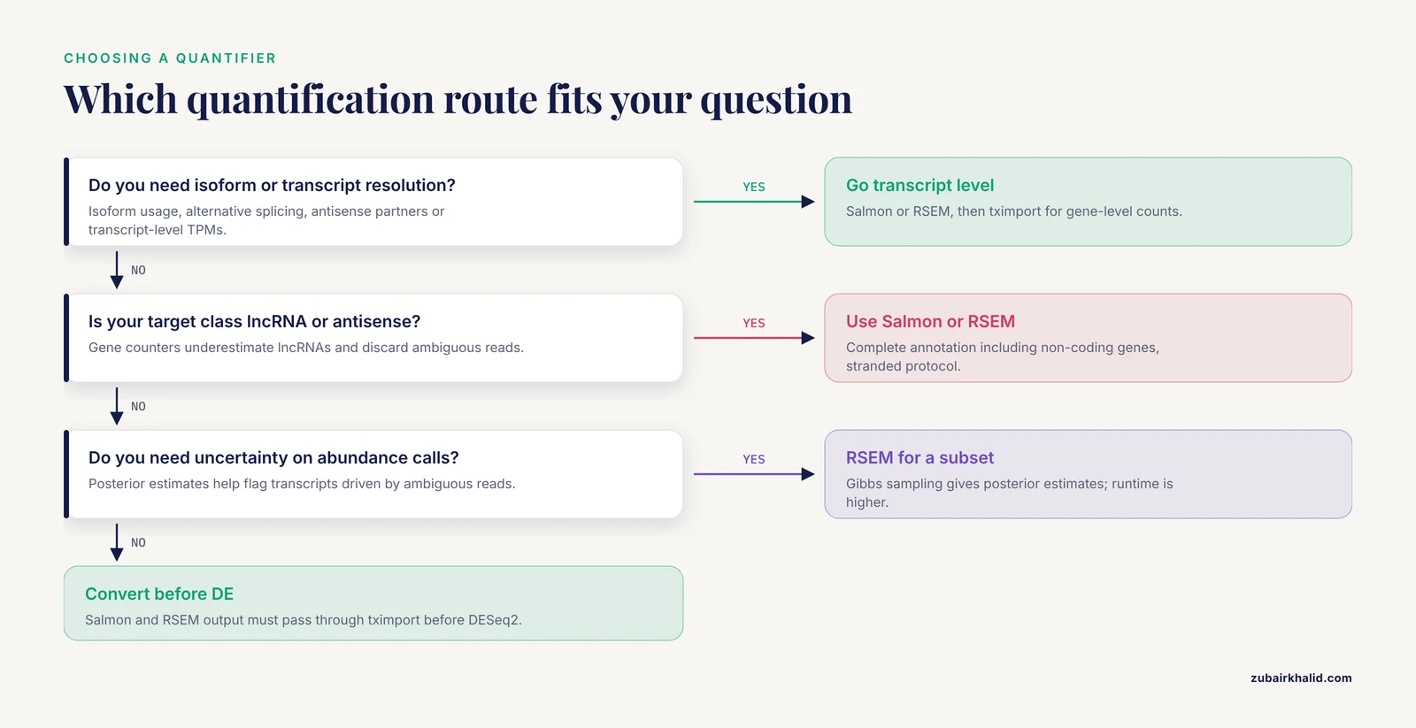
Reading the benchmark literature and official documentation, five criteria come up repeatedly as the ones that actually change the answer.
1. What unit of analysis do you need?
If your question is "which genes are differentially expressed," any of the three can get you there, and gene-level counts from featureCounts are the conventional, well-trodden path. If your question touches isoforms, alternative splicing, transcript usage, or genes with antisense partners, you need transcript-level quantification from Salmon or RSEM.
2. How well annotated is your organism?
Quantification is bounded by the annotation file. Full transcriptome annotation that includes both protein-coding and non-coding RNAs greatly improves the specificity of expression estimates, and this is especially true for non-coding transcripts [1]. A stale GTF that lacks recent lncRNA models will cause featureCounts to undercount those genes no matter how well the tool itself performs. The corollary from the same benchmark is that pseudoalignment and RSEM methods, which quantify against the complete transcript reference, tolerate complex annotations better than overlap counters [1].
3. Does your library type and target gene class demand it?
Unstranded data cannot distinguish antisense transcripts from their sense partners. Antisense lncRNAs are poorly quantified by gene-count methods in unstranded protocols, and the problem is substantially improved with stranded library preparation and stranded-aware quantification settings [1]. If your experiment involves antisense or overlapping transcription, use a stranded protocol and verify that your tool is configured for it.
4. Do you need uncertainty?
Salmon offers bootstrapping, and RSEM offers Gibbs-sampling-based posterior estimates. Both let you attach credible intervals to abundance estimates, which matters when you want to flag transcripts whose apparent differential expression is driven by ambiguous read assignment rather than real biology. Overlap counters offer no such estimate.
5. What can your downstream analysis consume?
DESeq2 and edgeR model negative binomial counts and expect raw integer counts. featureCounts output drops straight in. Salmon and RSEM output needs tximport to produce gene-level counts on the corrected scale. This is a convenience difference, not a barrier, but pipelines that skip the conversion step produce statistically invalid DE results.
Worked Scenarios
Scenario A: Bulk mRNA differential expression in human tissue, 24 samples. You have stranded poly(A) libraries, a well-annotated reference, and the goal is a ranked list of differentially expressed genes. Align with a splice-aware aligner, count with featureCounts using the correct strandedness flag, and run DESeq2. This is the fastest defensible pipeline, and every step is easy to explain to a reviewer.
Scenario B: lncRNA and antisense transcript analysis. Your question involves long non-coding RNAs. The benchmark evidence is direct here: pseudoalignment methods (Kallisto, Salmon) and RSEM outperformed HTSeq and featureCounts for lncRNA quantification at both sample- and gene-level comparisons, detected more lncRNAs, and correlated more highly with simulated ground truth, while HTSeq and featureCounts often underestimated lncRNA expression [1]. Use a complete annotation including non-coding genes, quantify with Salmon or RSEM, and be certain the protocol was stranded.
Scenario C: Isoform usage in a large cohort, 300+ samples. You need per-sample transcript TPMs, and the compute budget is tight. Salmon was built for exactly this, quantifying hundreds of samples per hour on a single node without an alignment step, and its quasi-mapping accuracy tracks closely with RSEM in benchmark comparisons [1]. Reserve RSEM for a subset where you need posterior uncertainty.
Scenario D: Non-model organism with an incomplete annotation. When the transcriptome reference contains predicted transcripts, bias correction in Salmon and careful QC of the annotation matter more than the choice between aligner flavors. In completely unannotated species, small RNA workflows built in tools like Galaxy have shown that combining orthologue information from related species with mapping to other non-coding RNAs prevents falsely annotated microRNAs, a principle that applies to mRNA annotation curation as well [2].
Genes, Transcripts, and the Downstream Analysis Handoff
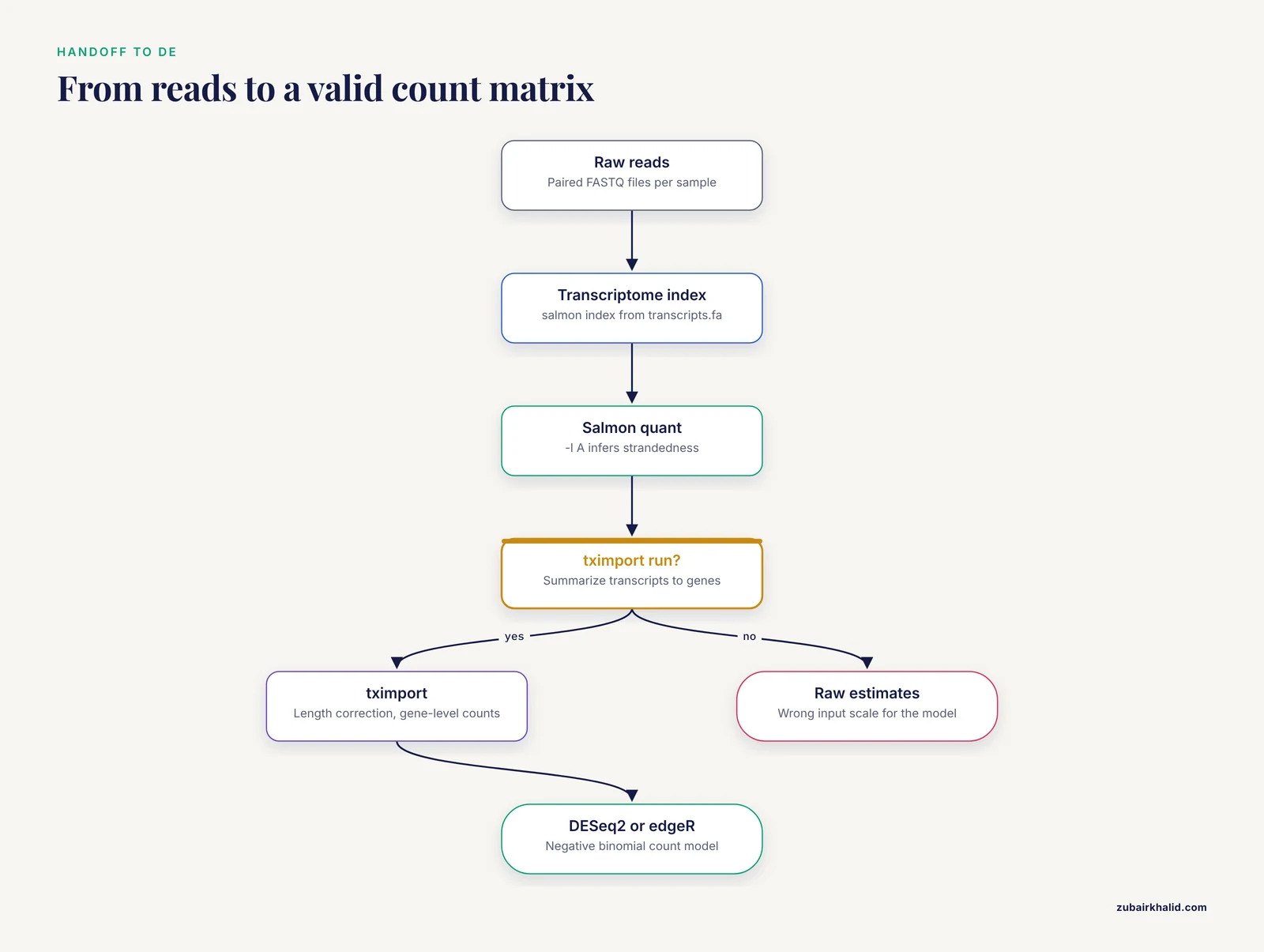
Most RNA-seq papers report at the gene level, and most differential expression tools operate at the gene level. That creates a persistent handoff problem for transcript-level quantifiers, and the standard solution is tximport.
The tximport workflow reads Salmon or RSEM output, summarizes transcripts to genes, corrects for changes in isoform length across samples (which otherwise distort gene-level summaries), and produces a count matrix on a scale that DESeq2 and edgeR accept. It also preserves the original transcript TPMs for analyses that need them. If you quantify with Salmon and then run DESeq2, tximport is not optional. Using raw Salmon estimated counts directly gives the DE model the wrong input scale.
One more subtlety: differential transcript expression and differential gene expression are different questions. A gene can be constant in total expression while its isoform proportions change completely. If isoform switching is your hypothesis, analyze transcript-level outputs with tools built for transcript usage, not a gene-level DE pipeline.
Upstream Alignment: STAR, HISAT2, and Subread
Even though Salmon skips genome alignment, most pipelines that use featureCounts or RSEM need a spliced aligner upstream. The three mainstream options are STAR, HISAT2, and Subread. The lncRNA benchmark applied each of these aligners in combination with each quantification tool and found that the quantification strategy, not the aligner choice, drove the largest differences in accuracy [1]. That is a useful simplification: pick an aligner you can run efficiently and reproduce, and spend your optimization effort on the quantification step and the annotation.
When alignment is required, the essential QC outputs are mapping rate, fraction of uniquely mapped reads, and splice junction support. A low mapping rate usually indicates contamination, wrong reference build, or a read length mismatch, and no quantification tool can rescue bad input.
Building Quantification Pipelines with a Workflow Manager
A quantification step in isolation is easy. A quantification step run consistently across hundreds of samples, with correct metadata, software versions, and logs, is what separates reliable analysis from chaos. That consistency problem is why nearly every modern RNA-seq pipeline runs under a bioinformatics workflow manager.
Nextflow vs Snakemake
Nextflow and Snakemake are the two dominant open-source workflow managers for bioinformatics, and the nextflow vs snakemake question comes up in every lab considering a new pipeline.
Nextflow is written in a Groovy-based DSL and emphasizes containers, cloud execution, and long-running process supervision. Its strengths are native support for Docker and Singularity containers, automatic resume of failed jobs from the last successful task, and mature integration with cloud platforms and cluster schedulers. Public bioinformatics pipelines such as nf-core are built on it, and its execution model handles restarts and retries gracefully.
Snakemake is Python-based and structures pipelines as a directed acyclic graph of rules mapping input files to output files. Its strengths are approachability for Python-centric labs, easy integration with conda environments for software pinning, and a rule model that is intuitive when your pipeline is a chain of file transformations.
For quantification pipelines specifically, both managers handle the task equally well. The honest difference is operational. If your group leans Python and runs mostly on a local cluster or workstation, Snakemake with conda is often the shorter learning curve. If your samples live on heterogeneous compute, you need containerized reproducibility guarantees, or you want to reuse community-maintained pipelines, Nextflow's execution model pays off. The wrong choice is not either tool, it is writing no workflow at all and running commands by hand.
Galaxy, BRC-Analytics, and Agentic Interfaces
Not every lab should maintain a Nextflow or Snakemake installation. Recent work on standardizing RNA-seq analysis for fungal pathogens demonstrated a framework combining public data repositories, a Galaxy-based analysis platform (BRC-Analytics), and agentic AI assistance, with the constraint that AI agents invoke Galaxy's native tools rather than manipulating data directly, preserving full provenance, and achieved near-perfect correlation with published results despite annotation version differences [3]. The lesson generalizes: a well-instrumented, tool-level workflow system enforces reproducibility even when the interface is conversational, and standalone notebooks can reproduce the analysis outside the AI layer when needed [3].
R-Based Workflow Environments
For R-centric teams, systemPipeR provides an R/Bioconductor environment for building and running end-to-end NGS workflows with automated report generation, a uniform workflow interface across applications, flexible sample annotation handling, and support for running both R and command-line software on local computers and clusters [4]. Quantification steps such as featureCounts and transcript quantifiers slot into it as command-line steps called from R, and the report generation is genuinely useful for producing per-run QC documents.
Reproducibility Beyond Tool Choice
Whatever manager you use, three practices carry most of the reproducibility value for quantification:
- Pin software versions in containers or conda environments, and record the exact versions in the run log.
- Freeze the annotation and genome build versions in the pipeline configuration, because a GTF update changes counts even when nothing else changes.
- Capture per-sample statistics such as read counts in and counts out at every step, so silent failures surface as outliers.
Quantification in Specialty Library Types
The bulk RNA-seq framework above does not transfer unchanged to every library type, and knowing where it breaks is part of a complete quantification strategy.
Small RNA and miRNA isoforms. microRNA libraries are 18 to 30 nucleotide reads, and a substantial fraction of miRNA expression exists as isomiRs, variants of the canonical miRNA sequence. Dedicated small RNA pipelines that assemble embryo- and species-specific miRNA catalogs and quantify isoforms explicitly, rather than collapsing everything to the canonical sequence, revealed large numbers of rare isoforms and species-conserved novel miRNAs that generic pipelines miss [2]. Never push small RNA data through a bulk mRNA quantifier.
Single-cell droplet data. Droplet single-cell RNA-seq methods such as those built on dissolvable hydrogel beads use cell and UMI barcodes, and quantification collapses barcodes to cells rather than genes per sample. Open-source droplet platforms have demonstrated throughput and sensitivity comparable to commercial assays, generating several thousand single-cell transcriptomes from flash-frozen tissue in a single run [5]. Specialized quantifiers handle the barcode structure, and the quantification output is a cell-by-gene matrix rather than a sample-by-gene matrix.
Full-length single-cell data. Full-length single-cell protocols such as Smart-seq derivatives and FLASH-seq capture entire transcripts rather than just 3-prime ends, which makes them suitable for isoform-level analysis that 3-prime droplet data cannot support [6].
Long-read single-cell data. Benchtop single-cell long-read platforms that couple molecular barcoding with Oxford Nanopore sequencing enable isoform-resolved measurement from thousands of individual cells, requiring pipelines built for barcode recovery, alignment, and transcript quantification of full-length reads [7]. The quantification logic differs from short-read Salmon or RSEM because the reads themselves span full isoforms.
Nuclear RNA-seq. Single-nucleus RNA-seq from frozen tissue has its own quantification considerations, including intronic read handling, and published workflow templates for reanalyzing public single-nuclei datasets have been used to characterize cell subtype diversity in adipose tissue under thermogenic challenge [8].
Polyadenylation site data. 10x-style scRNA-seq captures RNA 3-prime ends, and reads that include the non-templated polyA tail provide direct evidence of cleavage and polyadenylation sites. The PolyASite atlas was constructed by mining this signal from a large compendium of public scRNA-seq datasets, aggregating samples by tissue of origin to build tissue-level catalogs with stringency levels that let users balance sensitivity and specificity [9]. This is a useful reminder that quantification output can feed secondary analyses well beyond expression matrices.
Clinical and precision oncology settings. RNA-seq is increasingly incorporated into clinical tumor profiling, where quantification quality directly affects calls on oncogene overexpression, gene fusions, splice variants, RNA-based variant calling, and oncoviral gene expression [10]. Clinical pipelines demand locked software versions, explicit strandedness, and validated annotation releases, because the cost of a quantification error is a patient report rather than a rejected manuscript.
Benchmarking Your Own Pipeline
Published benchmarks are a starting point, not a substitute for checking your own data. A curated benchmarking resource, Dex-Benchmark, provides datasets and code templates for evaluating transcriptomics tools against dexamethasone perturbation data with known expected associations, including optimization of data processing strategies for chemical perturbations and CRISPR single-gene knockdown experiments [11]. The general approach transfers to any pipeline: run two quantification strategies on the same data, check the correlation of the results, and look at where they disagree rather than only at summary statistics.
A practical self-check for your own quantification takes under an hour:
- Quantify one representative sample with featureCounts and with Salmon.
- Convert both to gene-level counts and compute the correlation of log counts.
- List genes where the two methods differ by more than a threshold, and inspect their annotations for overlap, paralogy, or antisense structure.
- Check strandedness by verifying that read assignments agree with the expected library type.
Disagreements concentrated at overlapping or antisense loci are expected and confirm the benchmark literature [1]. Disagreements everywhere suggest a configuration error, most often strandedness.
Common Mistakes and Limitations
- Wrong strandedness flag. Setting the wrong library orientation reverses assignments on antisense transcripts and is silent in the output. Run Salmon with library type auto-inference as a check, or verify against a known single-isoform housekeeping gene.
- Quantifying lncRNAs with gene counters. featureCounts and HTSeq underestimate lncRNA expression and detect fewer lncRNAs than Salmon, Kallisto, or RSEM, especially for antisense lncRNAs in unstranded data [1]. If your hypothesis involves non-coding transcripts, this is a first-order error, not a rounding difference.
- Using stale or incomplete annotations. Quantification cannot see transcripts missing from the reference. Update the GTF with every pipeline release and record the version.
- Treating TPM as fold-change input. TPM is for within-sample comparisons of relative abundance. Differential expression tools need counts. Feeding TPM into a count model inflates variance estimates and produces false confidence.
- Skipping tximport after Salmon or RSEM. Raw transcript-level estimated counts are not a valid DESeq2 input. Summarize to gene level with length correction first.
- Comparing pipelines across annotation versions. A reanalysis of published fungal RNA-seq data achieved near-perfect correlation with original results despite annotation version differences, but only because the framework controlled for reference and tool versions explicitly [3]. Without that control, annotation drift masquerades as biological signal.
- Assuming the aligner is the variable. Benchmark evidence shows the quantification method, not the aligner, drives the largest differences in accuracy [1]. Teams that spend weeks tuning STAR parameters while ignoring quantification choices are optimizing the wrong component.
- Forgetting that ambiguity is biological. Reads discarded at multi-gene loci are not noise. They are often the most informative reads about alternative splicing and antisense transcription.
- Running manual pipelines without a workflow manager. Re-running a hand-executed pipeline months later rarely reproduces it exactly. Pin versions, use Nextflow, Snakemake, or a managed environment, and log everything.
- Individual-case caveat. Any specific research or clinical interpretation depends on the individual sample, protocol, and question, and should be reviewed with a qualified specialist rather than generalized from a pipeline default.
Frequently Asked Questions
Which is the best RNA-seq quantification tool, featureCounts, Salmon, or RSEM?
There is no single best tool, only the best fit for your question. For straightforward gene-level differential expression in a well-annotated organism, featureCounts is fast, transparent, and conventional. For transcript-level or isoform-level questions, Salmon and RSEM are better, and for long non-coding RNA quantification specifically, Salmon, Kallisto, and RSEM outperform featureCounts and HTSeq in benchmark comparisons [1]. The most defensible answer is to quantify with one method that matches your primary question and validate a subset with a second method.
Do I still need a genome aligner if I use Salmon?
No, Salmon quantifies directly against a transcriptome index without genome alignment, which is one of its main speed advantages. A genome alignment is still needed if your goals include novel transcript or splice junction discovery, or if you want to inspect reads in genomic context. Many pipelines run Salmon for quantification and a genome alignment only for QC and exploratory views.
Can I use Salmon or RSEM output with DESeq2?
Yes, but not directly. Pass the transcript-level estimates through tximport, which summarizes transcripts to genes, corrects for isoform length changes between samples, and produces a count matrix on the scale DESeq2 and edgeR expect. Using raw estimated counts without this step gives invalid statistical results.
Nextflow vs Snakemake, which workflow manager should I pick?
Both manage reproducible RNA-seq pipelines equally well at the task level. Choose Nextflow when you need containerized execution across clusters or clouds, automatic job resumption, and access to community pipelines built on it. Choose Snakemake when your team is Python-centric, your compute is local, and you prefer conda-based software pinning with a file-based rule model. Pick the one that fits your infrastructure and team skills, and never rely on manual execution for anything you may need to reproduce.
Does quantification choice matter for lncRNA and antisense transcripts?
Yes, substantially. A direct benchmark found that pseudoalignment methods and RSEM detect more lncRNAs and correlate better with simulated ground truth than HTSeq and featureCounts, which often underestimate lncRNA expression, and that antisense lncRNAs in particular are poorly quantified by gene-count methods unless the protocol is stranded [1]. For non-coding and antisense targets, use Salmon, Kallisto, or RSEM with a complete annotation and stranded data.
Can I mix tools within one pipeline, for example Salmon for transcripts and featureCounts for genes?
Yes, and it is a reasonable strategy. Running featureCounts for a conventional gene-level DE matrix alongside Salmon for transcript-level analysis gives you the strengths of both, at the cost of running two quantification steps per sample. The two outputs should agree closely at stable protein-coding genes, and where they diverge, the divergence is informative about annotation complexity at that locus.
Sources
- Benchmark of long non-coding RNA quantification for RNA sequencing of cancer samples.
- Small RNA-seq analysis of single porcine blastocysts revealed that maternal estradiol-17beta exposure does not affect miRNA isoform (isomiR) expression.
- Standardizing RNA-seq Analysis of Fungal Pathogens Using BRC-Analytics and Agentic AI: A Candidozyma auris Case Study.
- systemPipeR: NGS workflow and report generation environment.
- Hydrop enables droplet-based single-cell ATAC-seq and single-cell RNA-seq using dissolvable hydrogel beads.
- Full-Length Single-Cell RNA-Sequencing with FLASH-seq.
- BenchDrop-seq: a microfluidics-free platform for benchtop single-cell long-read RNA sequencing.
- Multidimensional Single-Nuclei RNA-Seq Reconstruction of Adipose Tissue Reveals Adipocyte Plasticity Underlying Thermogenic Response.
- PolyASite v3.0: a multi-species atlas of polyadenylation sites inferred from single-cell RNA-sequencing data.
- The actionable transcriptome: a framework for incorporating RNA sequencing into precision oncology.
- Dex-Benchmark: datasets and code to evaluate algorithms for transcriptomics data analysis.