How to Find and Download RNA-Seq Data for Non-Model Organisms on NCBI
By Dr. Zubair Khalid, DVM, MS, PhD ·

Raw RNA-seq reads live in the Sequence Read Archive (SRA), processed expression matrices live in the Gene Expression Omnibus (GEO), and the study-level context that ties both together lives in BioProject and BioSample. Rule of thumb for non-model organisms: start your search in BioProject or the main NCBI search box, confirm the raw reads exist in SRA, then check GEO for processed counts you can compare against. Journal data policies push nearly every modern transcriptome study into NCBI, which makes it the single most productive place to find RNA-seq data for non-model organisms, even for species with no genome assembly at all [1].
This guide walks through how to use NCBI for this task, compares the main rna-seq data for non-model organisms ncbi options, explains their pros and cons, and gives concrete commands you can run today.
How NCBI Organizes Transcriptome Data
Understanding the database structure saves hours of frustrated searching. NCBI is not one database. It is a set of interconnected databases, each holding a different layer of the same study, linked by accessions.
The accessions themselves tell you where you are:
- PRJNA… (BioProject): the umbrella record for an entire study. It holds the study description, the submitter, the linked publication, and links down to every sample and every run.
- SAMN… (BioSample): one biological sample, with attributes such as tissue, developmental stage, treatment, and collection details.
- SRR… (SRA run): one sequencing run, the unit that maps to a single FASTQ file (or a pair of files for paired-end data).
- GSE… (GEO Series) and GSM… (GEO Sample): processed data organized as a study, often with normalized count tables and linked raw reads in SRA,, [4].
- GHP#… or GB#… (TSA): transcriptome shotgun assemblies, that is, de novo assembled transcripts submitted by researchers working on organisms without a reference genome [1].
The hierarchy flows in one direction. A BioProject contains BioSamples, and BioSamples contain SRA runs. GEO sits partially parallel to this, because a GEO Series can hold its own processed files while pointing to SRA for the raw reads. A typical published dataset, such as the single-cell renal papilla study with BioProject PRJNA735197 and GEO accession GSE176155, shows both layers linked to each other [5].
For a non-model organism, this structure matters more than it does for mouse or human, because you often need to evaluate whether the organism has a reference assembly, whether transcripts have been assembled before, and what metadata describes each sample. You gather all of that from the linked records rather than from a single page.
The Main NCBI Options for Non-Model RNA-Seq Data
The table below is the core comparison. Each option is then explained on its own terms.
| Database | What it holds | Best for | Main caveat |
|---|---|---|---|
| SRA (Sequence Read Archive) | Raw sequencing reads in FASTQ or aligned formats | Reanalysis from scratch, de novo assembly, new pipelines | Large downloads, variable quality, metadata quality varies by submitter [1], [6] |
| GEO | Processed data such as count matrices, plus links to raw reads | Quick differential expression reanalysis, meta-analyses across studies [2], [7] | Not every series provides counts, and library details may be sparse |
| BioProject / BioSample | Study descriptions, sample metadata, links to runs and publications | Planning your analysis, confirming sample design, batch downloads | Holds no sequence data itself, it is a signpost layer |
| TSA (Transcriptome Shotgun Assembly) | Assembled transcript contigs from RNA-seq | When you need a transcript reference for an organism without a genome [1] | Assemblies differ in quality and completeness between submissions |
| Assembly / RefSeq Genome | Reference genomes and gene annotations | Alignment-based analysis when a genome exists for your species or a close relative [8], [9] | Annotation for non-model species is often largely computational prediction with little experimental support [9] |
| NCBI Datasets | Bulk genome and annotation downloads | Fetching reference FASTA and GFF files for many species at once | Focused on genomes, not expression data |
SRA: The Raw Reads
The Sequence Read Archive is where virtually every RNA-seq experiment lands eventually, because journals require data availability and SRA is the dominant deposition site [1]. For small RNA studies alone, SRA hosts miRNA-seq data for more than 800 different species, which illustrates how broad the taxonomic coverage has become [10]. If reads were produced for a non-model organism, they are almost certainly here, whether the species is an apple snail [11], an olive fruit fly [12], or a medicinal plant [13].
The strength of SRA is completeness. You get the actual reads, in original orientation, with the original quality scores, so you can apply your own quality control, trimming, alignment, and counting rather than trusting someone else's pipeline [6], [14]. The weaknesses are size and inconsistency. A single Illumina lane can run to tens of gigabytes, metadata fields are only as complete as the submitter made them, and raw reads sometimes reveal quality problems the original paper never mentioned.
One detail worth checking early is the library strategy. Within SRA, standard mRNA profiling is indexed under "RNA-Seq", while small RNA profiling appears under "miRNA-Seq", and these need different downstream tools and annotation databases [10].
GEO: The Processed Layer
GEO organizes data as Series (GSE) with Samples (GSM), and many depositors upload count matrices, FPKM or TPM tables, and differential expression results as supplementary files [3], [4]. Secondary analyses of public transcriptomic data frequently work directly from GEO, pooling multiple datasets to find consistent signatures across cohorts [2], [7].
The appeal for non-model organisms is speed. If a GEO Series ships a raw count matrix, you can move straight to differential expression and enrichment analysis without downloading, trimming, and aligning hundreds of gigabytes of reads. The risk is transparency. A count matrix does not tell you which transcript reference was used, how ambiguous multimappers were handled, or whether strandedness was counted correctly. When those details matter, and for non-model organisms they usually do, you end up going back to SRA anyway.
BioProject and BioSample: The Context Layer
BioProject records answer the questions that decide whether a dataset is usable. How many biological replicates were there? What tissue, what stage, what treatment? Is there a linked publication? For example, a maize dataset described in a Data Brief lays out two inbred lines, a hybrid, two watering regimes, mycorrhizal inoculation, and three biological replicates per genotype-by-treatment combination, all readable from the study record before you download a single file [15].
BioSample records carry the per-sample attributes. On well-curated submissions you can read tissue, developmental stage, and condition directly. On careless submissions the fields say "RNA" or "sample from whole body", and you have to recover meaning from the paper. This variability is one of the real pros and cons you weigh when picking between options.
TSA: Assembled Transcripts When No Genome Exists
For species without a reference genome, the Transcriptome Shotgun Assembly database holds de novo assembled transcript contigs submitted by other researchers [1]. These assemblies serve two purposes. They can be your reference for read mapping and quantification, and they can be a source of sequences for designing primers or building protein databases from unsequenced organisms, an approach demonstrated for tree nut allergen detection [16].
TSA assemblies are not standardized. One group may assemble 43,413 transcripts for a plant with 95 percent of them annotated against NCBI's green plant database [13], while another submission for a related species may be far less complete. Treat each assembly as a candidate reference to evaluate, not a finished product.
Assembly and RefSeq: The Reference Layer
If your organism has a genome assembly, alignment-based RNA-seq analysis becomes possible, and the quality of the gene annotation becomes the limiting factor. The horse genome illustrates the problem. Most horse gene models are known only by projection from other species, most annotated genes are single-transcript, and one reanalysis of 561 RNA-seq samples found 7,531 transcripts not associated with any annotated horse gene [9]. The same pattern repeats across mammals and plants with incomplete annotation [17], [13].
NCBI Datasets provides a straightforward way to pull the genome FASTA and annotation GFF for your species, or for a close relative you plan to use as a proxy reference.
Step-by-Step Search Workflow
Step 1: Pin Down the Organism Name
Taxonomic naming errors are the most common reason searches come back empty. Synonyms, old names, and misspellings all break exact queries. Open the NCBI Taxonomy database, type the organism name, and confirm the scientific name and its taxonomy ID. For example, searching Cassia angustifolia leads you to senna, a drought-tolerant legume studied by transcriptomics precisely because public data were sparse [13]. Keep the taxonomy ID, because some tools and filters work better with the numeric ID than with names.
Step 2: Search BioProject for Study-Level Records
In the NCBI search box or at the BioProject database directly, search the organism name and add terms such as "RNA-Seq", "transcriptome", or the treatment you care about. A query like Bactrocera oleae AND transcriptome returns the BioProject behind the nanopore embryo study for that olive pest, including the 31 million MinION reads and the improved transcriptome assembly built from them [12].
Open the candidate BioProject and read three things: the study abstract, the linked publication, and the scope table showing how many BioSamples and SRA runs it contains. If the counts look right, proceed. If the project lists zero SRA runs, the raw data may be on hold or hosted elsewhere.
Step 3: Move to SRA and Use the Run Selector
From the BioProject page, follow the link to its SRA experiments. The Run Selector is the tool that makes hundreds of runs manageable. Its left panel provides facets you can combine:
- Organism, to filter within multi-species submissions
- Library strategy, to separate "RNA-Seq" from "miRNA-Seq" and other assays [10]
- Platform, to separate Illumina from PacBio and Oxford Nanopore runs [12]
- Layout, to isolate paired-end from single-end libraries
- AvgLength and MBases, to spot degenerate or truncated runs before downloading
Click through two or three runs to their BioSample records and confirm the metadata matches what the paper describes. A dataset only supports your analysis if the sample labels align with the biological conditions in the publication.
Step 4: Check GEO for Processed Files
Search GEO for the organism name and your keywords. When a Series exists, the page lists supplementary files, which frequently include count matrices and normalized tables,. Compare the GEO sample table against the SRA runs to confirm the two records describe the same experiment. Secondary analysis studies routinely harvest multiple GEO datasets this way, for example pooling seven public pancreatic cancer series with a new cohort to find consistently dysregulated hub genes [7].
Step 5: Record the Accessions You Need
Before downloading anything, write down the BioProject, the SRA run list, and the GEO accession if one exists. Reproducibility starts here. A short accessions block in your analysis notebook, listing exactly which SRR runs belong to which condition, prevents the most common reanalysis mistake, which is losing track of which file is which sample.
How to Download the Data
Browser Downloads
For a handful of runs, the SRA Run Browser offers a direct download of the FASTQ or the SRA format file. GEO supplementary files download over HTTPS from the Series page. This route is fine for pilot work but painful for anything over a few gigabytes.
SRA Toolkit: The Standard Route
The SRA Toolkit is the standard command-line path, and published RNA-seq workflows built for cloud notebooks and local machines alike use it as the first step [6], [14]. The two commands that matter are:
prefetch SRR21619922
fasterq-dump SRR21619922 --split-files --threads 8
gzip SRR21619922_1.fastq SRR21619922_2.fastq
prefetch pulls the run from SRA into local storage. fasterq-dump converts it to FASTQ, and -split-files separates paired-end data into forward and reverse files. Forgetting -split-files is a classic error that leaves you with one interleaved file and a confusing alignment step downstream. For a whole study, loop over a list of accessions:
while read acc; do prefetch "$acc" && fasterq-dump "$acc" --split-files --threads 8; done < srr_list.txtBulk and Programmatic Routes
For dozens or hundreds of runs, request the file list from an SRA project page, or use E-utilities to script the retrieval:
esearch -db sra -query "PRJNA735197" | efetch -format runinfo > runinfo.csvThis produces a table of every run in the project with its sample, layout, platform, and size, which doubles as your sample sheet for downstream analysis. Pipeline developers rely on exactly this kind of scripted retrieval, as the PipeSeq pipeline for Chlamydomonas reinhardtii demonstrates by pulling raw RNA-seq sets from NCBI SRA through SRA Toolkit before alignment and differential expression [6]. For genomes and annotations rather than reads, NCBI Datasets offers both a web interface and a command-line tool for bulk retrieval.
GEO Files
On a GEO Series page, the "Supplementary file" links lead to processed tables. A structured workflow for limited-resource environments shows the typical sequence after retrieval: download from NCBI GEO or SRA, quality check with FastQC, trim with Trimmomatic, align with HISAT2, count with featureCounts, and test differential expression with DESeq2, all runnable in free cloud notebooks [14]. That pipeline was written for mammalian data, but the same shape applies to any organism with a reference transcriptome.
Choosing the Best RNA-Seq Data for Non-Model Organisms on NCBI
Accession hunting is easy. Deciding whether a dataset can actually answer your question takes more care. These criteria separate usable datasets from dead ends.
Experimental Design and Replication
Differential expression needs biological replication, and three replicates per condition is the common minimum you will see in deposited datasets, as in the maize mycorrhiza study with three biological replicates per genotype-by-treatment combination [15]. Check that the design matches your comparison. A dataset built to compare drought stages in leaves will not answer a question about root responses, no matter how well the reads were sequenced.
Library Type and Strandedness
Library preparation methods differ in ways that change the analysis. A QuantSeq 3' mRNA-seq library is strand-specific and concentrates reads at the transcript 3' end, which is excellent for gene-level counting on a known reference [15] but less suited to transcript isoform reconstruction. Standard stranded paired-end libraries support isoform work and strand-aware counting. Long-read platforms such as Oxford Nanopore produce full-length transcript information that short reads cannot, enabling de novo assembly and a fourfold increase in transcriptome diversity over existing annotations in the olive fruit fly study [12]. Check the library strategy and source fields in SRA before committing.
Reference Availability
This is the dividing line for non-model work. With a genome assembly and gene annotation, you align reads and count per gene [6], [14]. Without one, you either assemble transcripts de novo from the reads, as done for eight apple snail species from 1.2 billion Illumina reads yielding 20,730 to 35,828 unigenes per species [11], or you adapt someone else's TSA assembly [1]. Some non-model projects also benefit from deliberately mapping reads to a related reference, but the closer option is not always available.
Depth, Read Length, and Layout
Within the Run Selector, average read length and total bases per run give you a fast sense of whether a dataset has enough depth for your purpose. Expression profiling of well-annotated genes tolerates shallower sequencing than de novo assembly or isoform discovery, where depth and read length dominate assembly quality [12], [11].
Metadata Completeness
Read the BioSample attributes before downloading. Datasets with clear tissue, stage, and treatment labels, matched to a published description [15], [18], save days of reconstruction. Datasets with blank metadata fields force you to infer sample identities from file names, which is where reanalysis projects most often go wrong.
Annotation: The Special Problem of Non-Model Organisms
Finding and downloading the reads is half the workflow. Turning expression values into biological meaning requires functional annotation, and this is where non-model organisms punish the unprepared.
Common tools such as g:Profiler, DAVID, and GOrilla work well for well-annotated model organisms, but for bacteria and other microorganisms the curated functional annotations are often scarce, and the usual workaround is transferring annotations by homology through BLAST, which introduces annotation errors and can miss species-specific functions [8]. One practical remedy builds custom annotation R packages directly from NCBI genomic data, formatted for use with clusterProfiler, demonstrated on Mycobacterium tuberculosis H37Rv with public differential expression data [8]. For mammals, the Mammalian Annotation Database maps gene identifiers from less-annotated species to human homologs through gene symbols, Ensembl Compara orthology, and pairwise BLAST, which measurably improved enrichment results for a pig RNA-seq dataset [17].
Plant and animal studies without genome annotations rely on annotation transfer at scale. The senna drought transcriptome annotated 95 percent of its 43,413 assembled transcripts by BLASTX against the NCBI green plant database using taxonomy ID 33090, with top hits concentrated in soybean and other legumes [13]. The apple snail work similarly annotated 69.7 to 80.2 percent of unigenes per species against NCBI nr, Gene Ontology, and KEGG [11]. When you download reads from a species with no annotation, budget for this step, because the enrichment analysis at the end of the pipeline depends entirely on it.
The web of NCBI resources makes this easier than it sounds. Translated transcriptomes can even substitute for proteomes in some applications, as shown by protein database construction for unsequenced tree nuts, where a transcriptome-derived database performed comparably to the NCBI proteome for peptide identification [16].
Worked Scenarios
Scenario 1: An Ecologist Studying a Species With No Genome
You work on a gastropod with no genome assembly. Search NCBI Taxonomy to confirm the name, then search BioProject for "transcriptome" plus the genus. Suppose you find a project like the apple snail resource, which sequenced seven species and assembled de novo transcriptomes for eight, releasing thousands of unigenes with annotations against NCBI nr, GO, and KEGG [11]. Download the TSA assembly to use as your reference, download the raw runs from SRA for your own quantification, and plan a de novo or hybrid analysis. Your enrichment step will lean on homology annotation against better-studied relatives, with the caveats noted above [8], [17].
Scenario 2: A Crop Researcher Comparing Public Stress Datasets
You want to compare your own drought-stress RNA-seq in a crop against published work. GEO is your first stop, because Data Brief-style deposits often include count matrices and pathway statistics ready for reuse [3], [4]. Download the processed tables first, verify the design, and only fetch the raw SRA runs if you need to recount reads under your own pipeline. Check library details carefully, because a QuantSeq 3' dataset [15] and a standard stranded paired-end dataset [18] should not be merged into a single differential expression model without careful design.
Scenario 3: A Microbiologist Reanalyzing a Pathogen Dataset
You want the differential expression response of Mycobacterium tuberculosis H37Rv to rifampicin. Search GEO for the accession, confirm the six-sample design, and note that enrichment analysis for such organisms requires custom annotation resources built from NCBI data, as the published workflow does [8]. Fetch the raw runs from SRA with the toolkit, run the alignment-counting-differential expression chain, and use the custom annotation package for clusterProfiler-based enrichment [8], [6].
Scenario 4: A Small RNA Study Across Species
You are profiling miRNAs in a species outside the usual model set. Search SRA with the library strategy filter set to miRNA-seq. The coverage is broad, with data for more than 800 species hosted in SRA [10], and dedicated tools handle annotation for metazoan and plant small RNAs using curated databases and hundreds of reference assemblies [10]. Standard mRNA pipelines will not work here, so confirm the assay type before downloading.
Weighing the Options: Pros and Cons in Practice
The rna-seq data for non-model organisms ncbi options trade speed against control:
- SRA raw reads give you full control and are always the fallback, at the cost of download size and pipeline work [6], [14].
- GEO processed data give you speed and are ideal for cross-study comparisons,, at the cost of trusting the depositor's processing decisions.
- TSA assemblies give you a ready transcript reference for genome-free species [1], at the cost of uneven assembly quality.
- Assembly and RefSeq records give you alignment-based rigor where genomes exist [8], at the cost of annotation quality that is often prediction-heavy for non-model species [9].
Most real projects use two or three of these together, which is why starting from BioProject, which links all of them, is the practical default.
Common Mistakes and Limitations
Confusing accession types. SRR, SRS, SRX, PRJNA, and GSE numbers all identify different layers. Downloading "the study" by its BioSample accession or quoting a run accession in a paper as if it were the project are frequent, avoidable errors. Record the BioProject as the primary citation for the dataset.
Forgetting paired-end handling. Converting SRA files without -split-files produces a single file that breaks downstream tools expecting mate pairs [14]. The same class of error appears when people treat single-end and paired-end samples as interchangeable within one count matrix.
Merging processed data across studies without harmonization. Different pipelines, different reference builds, and different library protocols produce counts that are not directly comparable. Cross-study GEO analyses that pool datasets succeed when they reprocess carefully or use consistent normalization, not by naively concatenating matrices [2], [7].
Trusting predicted annotation blindly. For many non-model species, most gene models are computational projections with little experimental support [9], and homology-based annotation transfer can introduce errors and miss species-specific functions [8]. Treat annotation as a hypothesis layer, and validate key genes where the study allows.
Ignoring data holds and embargoes. Some BioProjects show sample and run counts but block downloads until a publication date. If the raw data are missing, check the project description for an expected release rather than assuming the data were never submitted [1].
Skipping library-strategy checks. Downloading a miRNA-seq run into an mRNA pipeline, or a 3' end-counting library into a splice-aware whole-transcript workflow, produces numbers that look plausible and mean little [10],.
Assuming the TSA or GEO layers match the raw reads. Assemblies and count matrices were built with specific parameters and references. If you reassemble or recount, your gene numbers will not match the paper's, and that is expected, not a bug.
The main limitation of any public-data reuse is that the experiment was designed for someone else's question. Replication, tissue selection, and sequencing depth were fixed by the original submitter, and no amount of reanalysis recovers a design that does not contain your comparison.
Frequently Asked Questions
What is the difference between SRA and GEO for RNA-seq data?
SRA stores raw sequencing reads, while GEO stores processed expression data such as count matrices alongside links to the raw reads. Start in GEO when you want ready-made counts, and go to SRA when you need the original FASTQ files to run your own pipeline [6], [14].
How do I download raw reads from SRA for a non-model organism?
Install SRA Toolkit, then run prefetch with the run accession followed by fasterq-dump with -split-files to produce paired FASTQ files [6], [14]. For whole projects, pull the run list with E-utilities or the Run Selector and loop the commands over all accessions.
Can I analyze RNA-seq data if my organism has no reference genome?
Yes, by de novo transcriptome assembly or by using a TSA assembly as the reference. Studies on apple snails, senna, and the northern wheatear all built usable transcriptomes from Illumina reads without a genome, annotating transcripts by homology against NCBI databases [11], [19], [13].
How do I judge whether a public dataset is good enough to reuse?
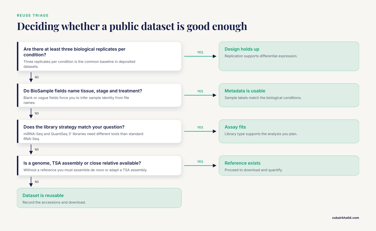
Check the BioProject for biological replication, read the BioSample metadata for tissue and treatment clarity, and inspect the Run Selector for layout, platform, and depth. Three biological replicates per condition is a common baseline in deposited datasets [15], and long-read or paired-end deep-sequenced datasets support more ambitious assemblies [12].
What is a BioProject accession and why should I start there?
A BioProject accession, formatted like PRJNA735197, is the umbrella record that links a study's description, publication, samples, and sequencing runs [5]. Starting there means you see the full design at once instead of stumbling onto disconnected runs.
How do I handle functional annotation for enrichment analysis in a non-model organism?
Options include homology-based transfer through BLAST against NCBI databases, mapping gene identifiers to a well-annotated species with tools such as the Mammalian Annotation Database, or building a custom annotation package from NCBI genomic data for use with clusterProfiler [8], [17], [13]. All rely to some degree on annotation transfer, so validate key findings independently.
Sources
- Good Citizenship Made Easy: A Step-by-Step Guide to Submitting RNA-Seq Data to NCBI.
- Identification of Potential Biomarkers in ASD Integrating RNA Seq Data and Machine Learning Approaches.
- A comparative transcriptomic dataset of hepatocytes derived from a panel of human induced pluripotent stem cells with different ethnicities as an in vitro population variability toxicity model.
- Transcriptomic data of larval zebrafish exposed to environmentally relevant levels of uranyl nitrate and sodium arsenite.
- Expression analysis of epithelial membrane protein 1 (EMP1) gene in kidney stone patients.
- Development and validation of the PipeSeq program for RNA-seq data analysis in the Chlamydomonas reinhardtii as a model.
- Dysregulated expression of cell cycle regulators CDC20, PLK1, BUB1, CDC45, CDCA5 in pancreatic ductal adenocarcinoma.
- Enhanced RNA-Seq Expression Profiling and Functional Enrichment in Non-model Organisms Using Custom Annotations.
- The transcriptome of equine peripheral blood mononuclear cells.
- sRNAbench and sRNAtoolbox 2022 update: accurate miRNA and sncRNA profiling for model and non-model organisms.
- AmpuBase: a transcriptome database for eight species of apple snails (Gastropoda: Ampullariidae).
- Nanopore long-read RNA-seq and absolute quantification delineate transcription dynamics in early embryo development of an insect pest.
- Exploring drought stress-regulated genes in senna (Cassia angustifolia Vahl.): a transcriptomic approach.
- Streamline Protocol for Bulk-RNA Sequencing: From Data Extraction to Expression Analysis.
- Illumina RNA-seq data of Genotype-specific responses of maize plants to Funneliformis mosseae.
- The Utility of Genomic and Transcriptomic Data in the Construction of Proxy Protein Sequence Databases for Unsequenced Tree Nuts.
- Mammalian Annotation Database for improved annotation and functional classification of Omics datasets from less well-annotated organisms.
- Transcriptome profile analysis of genes by RNA-sequencing in neonatal maternal separation rats with autistic-like behaviors.
- De novo annotation of the transcriptome of the Northern Wheatear (Oenanthe oenanthe).