How to Build a Real-Time Genomic Variant Calling Pipeline on AWS

By Dr. Zubair Khalid, DVM, MS, PhD · 2026-11-11

By the end of this article you will have a working real-time variant calling aws pipeline on AWS that accepts sequencing reads as they arrive, aligns them to a reference genome, calls variants, and writes the results to S3 without waiting for a full run to finish. You will be able to launch the infrastructure from the command line, process reads in chunks as they land, call variants with standard open source tools, and validate the output. The walkthrough uses a small bacterial genome so you can test the whole loop cheaply, then scales the same design to human data.

Here is what you need on hand before you start:

• An AWS account with permissions for S3, EC2, and IAM
• The AWS CLI version 2 installed and configured on your laptop (aws, version should return 2.x)
• A key pair for SSH access to your instances
• Roughly 5 GB of free disk space locally for a test reference and sample data
• Basic familiarity with the Unix shell

What "Real-Time" Means for Variant Calling

Traditional variant calling is a batch process. The sequencer finishes a run, you transfer a complete FASTQ file, you align every read, and only then do you call variants. Total latency equals sequencing time plus transfer time plus compute time.

Real-time analysis changes this. Reads stream off the instrument as they are produced. You process them in sequential chunks, so the first variant calls exist minutes after the first reads land rather than hours or days later. The genomic literature treats streaming as a first-class design pattern. Flint, a metagenomics profiling pipeline built on Apache Spark, streams sequencing reads so that profiling can begin while the sample is still being sequenced, and runs on Amazon's Elastic MapReduce service rather than on a local cluster [1]. The same architectural idea, chunked streaming compute on AWS, underlies every design in this article.

Two honest definitions of "real-time" apply to a variant calling aws pipeline:

1. Streaming latency. A chunk of reads arrives, and variant calls for that chunk appear within one or two chunk intervals. This is the mode this article builds.
2. Interactive latency. A clinician or researcher asks for an updated variant list at any moment, and the pipeline serves a current answer. This falls out of the first mode almost for free, because the latest merged VCF is always current to within one chunk.

Real-time does not mean the final call set equals the batch call set. Per-chunk calling has edge effects, which the Common Mistakes section covers in detail.

Architecture Overview

The pipeline has six components. The numbered list below shows the flow of data from instrument to answer.

1. Sequencer or upload client. An Illumina instrument, an Oxford Nanopore MinKNOW instance, or a simple script that pushes FASTQ chunks to S3. For testing, you upload chunks yourself with the AWS CLI.
2. S3 landing bucket. Raw reads arrive here in ordered chunks, named so that lexicographic sort equals chronological order.
3. Compute worker. One or more EC2 instances running bwa-mem2, samtools, and bcftools. For larger reference collections and higher throughput, the same roles can run on Amazon EMR with Spark, which is exactly how Flint achieves fast profiling against a very large collection of reference genomes [1].
4. Chunk processor. A shell script or small daemon on the worker that watches the landing location, picks up each complete chunk, and runs alignment plus calling on it.
5. Results bucket. Per-chunk and merged VCF files, BAM files, and logs.
6. Notification layer. An S3 event or a lightweight HTTP call that tells downstream consumers a new merged call set is available.

You can swap components later. Step Functions or AWS Batch can replace the simple watcher for production use, and an EMR cluster can replace the single EC2 worker when your reference collection grows beyond what one node holds in RAM. The step-by-step walkthrough below keeps every piece explicit so you can see what each service does before you abstract it away.

Step-by-Step: Building the Pipeline

Step 1: Create the Buckets and Configure Access

Open a terminal with your AWS credentials configured, then create two buckets. Use a region close to your sequencer.

aws configure set region us-east-1

aws s3 mb s3://my-lab-variant-raw
aws s3 mb s3://my-lab-variant-results

Expected output for each bucket command:

make_bucket: my-lab-variant-raw
make_bucket: my-lab-variant-results

Create a folder prefix for the run you are about to process. Chunk files must sort chronologically, so zero-pad the chunk index.

aws s3api put-object --bucket my-lab-variant-raw --key runA/000000/
aws s3api put-object --bucket my-lab-variant-raw --key runA/000001/

The zero-padding matters. Lexicographic order on 000001 through 000999 is correct, while 1 through 999 is not, and a watcher that sorts by name would process chunks out of order.

Step 2: Launch a Worker Instance

An m5.4xlarge (16 vCPU, 64 GB RAM) handles bacterial and small eukaryotic genomes comfortably and is a reasonable starting point for human data with bwa-mem2. Launch it with an Amazon Linux 2023 image. Get the latest AMI ID for your region first.

AMI=$(aws ec2 describe-images \
  --owners amazon \
  --filters "Name=name,Values=al2023-ami-2023.*-x86_64" \
  --query "sort_by(Images,&CreationDate)[-1].ImageId" \
  --output text)

aws ec2 run-instances \
  --image-id "$AMI" \
  --instance-type m5.4xlarge \
  --key-name my-key \
  --instance-initiated-shutdown-behavior terminate \
  --tag-specifications 'ResourceType=instance,Tags=[{Key=Name,Value=variant-worker}]'

Grab the public DNS name from aws ec2 describe-instances and connect.

ssh -i ~/.ssh/my-key.pem ec2-user@<PUBLIC_DNS>

If SSH fails with Permission denied (publickey), check two things. The .pem file must have permissions 600 (chmod 600 ~/.ssh/my-key.pem), and the key name passed to -key-name must match the key pair that exists in that specific region. Key pairs are regional resources, and a key pair created in us-west-2 does not exist in us-east-1.

Step 3: Install the Toolchain

Install the aligner, the SAM/BAM utilities, and the caller. Conda keeps versions pinned and reproducible.

sudo dnf install -y git curl wget
wget -qO- https://micromamba.snakepit.net/api/micromamba/linux-64/latest | tar -xvj bin/micromamba
./bin/micromamba create -y -n vcp -c conda-forge -c bioconda \
  bwa-mem2 samtools bcftools

Activate the environment and verify the versions.

micromamba activate vcp
bwa-mem2 version
samtools --version | head -1
bcftools --version | head -1

Expected output looks like this, with your own versions:

2.2.1
samtools 1.21
bcftools 1.21

Pin these versions in a text file committed to your repository. A variant calling pipeline that cannot state which aligner and caller produced a given VCF is not reproducible, and reproducibility problems usually surface months later during review.

Step 4: Prepare the Reference

For the cheap end-to-end test, use the E. coli K-12 reference. For human work, use GRCh38 and index it exactly the same way. Download and index:

mkdir -p ~/ref && cd ~/ref
wget https://ftp.ensemblgenomes.org/pub/bacteria/release-60/fasta/bacteria_0_collection/escherichia_coli_k_12_mg1655/dna/Escherichia_coli_k_12_mg1655.ASM584v2.dna.toplevel.fa.gz
gunzip Escherichia_coli_k_12_mg1655.ASM584v2.dna.toplevel.fa.gz
mv Escherichia_coli_k_12_mg1655.ASM584v2.dna.toplevel.fa ref.fa

bwa-mem2 index ref.fa
samtools faidx ref.fa

Expected output during indexing ends with lines like:

* Ref file: ref.fa
* Index file: ref.fa.bwt.2bit.64
Indexing completed in 0.63 CPU seconds, 0.63 real seconds

The .fai file created by samtools faidx is mandatory. bcftools refuses to call variants without it, and the failure message (Could not load the index for the reference) does not mention FASTA indexing, which is why this is one of the most common first-run errors.

Keep the reference build in the bucket next to the results so the exact reference used for any run is recoverable.

aws s3 cp ~/ref/ref.fa* s3://my-lab-variant-results/references/ecoli/ --recursive

Step 5: Load Test Data and Set Up Chunked Streaming

Download a public E. coli FASTQ set, split it into chunks of one million read pairs, and push the chunks to the landing bucket in order. Splitting on line counts works for FASTQ because every record is exactly four lines, so 4,000,000 lines equals one million pairs.

mkdir -p ~/data && cd ~/data
wget -q ftp://ftp.sra.ebi.ac.uk/vol1/fastq/SRR170/000/SRR1704700/SRR1704700_1.fastq.gz 2>/dev/null || \
wget -q https://ftp.sra.ebi.ac.uk/vol1/fastq/ERR066/000/ERR066087/ERR066087_1.fastq.gz
wget -q https://ftp.sra.ebi.ac.uk/vol1/fastq/ERR066/000/ERR066087/ERR066087_2.fastq.gz

# Decompress, split into 1M-pair chunks, recompress
for R in 1 2; do
  zcat ERR066087_${R}.fastq.gz > fq_${R}.tmp
  split -l 4000000 -d -a 4 fq_${R}.tmp chunk_${R}_
  for f in chunk_${R}_*; do gzip -f "$f"; done
  rm fq_${R}.tmp
done

Upload the chunks in paired order:

for i in $(seq -w 0 10); do
  aws s3 cp chunk_1_$i.fastq.gz s3://my-lab-variant-raw/runA/chunk_${i}_R1.fastq.gz
  aws s3 cp chunk_2_$i.fastq.gz s3://my-lab-variant-raw/runA/chunk_${i}_R2.fastq.gz
done

A note on scale. The streaming-with-chunks design scales cleanly. Flint streams reads against a 170 GB reference collection of 43,552 bacterial genomes from Ensembl and profiles one million Illumina paired-end reads against that collection on 64 machines in 67 seconds, roughly an order of magnitude faster than the prior state of the art while using a much larger reference [1]. Your chunk size and cluster size should be chosen so that processing one chunk takes less time than the sequencer takes to produce the next chunk. That single inequality is the whole capacity-planning problem.

Step 6: Write the Chunk Processor

Create a watcher script on the worker. It polls the landing prefix, grabs the next unprocessed chunk pair, and runs the full align-sort-call cycle on it.

Create ~/process_chunk.sh:

#!/bin/bash
set -euo pipefail

RAW=my-lab-variant-raw
OUT=my-lab-variant-results
RUN=runA
REF=/home/ec2-user/ref/ref.fa
WORK=/mnt/work
THREADS=14

CHUNK=$1
aws s3 cp s3://$RAW/$RUN/chunk_${CHUNK}_R1.fastq.gz $WORK/R1.fastq.gz
aws s3 cp s3://$RAW/$RUN/chunk_${CHUNK}_R2.fastq.gz $WORK/R2.fastq.gz

bwa-mem2 mem -t $THREADS $REF $WORK/R1.fastq.gz $WORK/R2.fastq.gz 2> $WORK/bwa.log \
  | samtools sort -@ 4 -o $WORK/chunk.bam -

bcftools mpileup -f $REF -q 20 -Q 20 -a AD,DP -Ou $WORK/chunk.bam \
  | bcftools call -mv -Oz -o $WORK/chunk.vcf.gz

bcftools index -t $WORK/chunk.vcf.gz
samtools index $WORK/chunk.bam

aws s3 cp $WORK/chunk.vcf.gz  s3://$OUT/$RUN/chunk_${CHUNK}.vcf.gz
aws s3 cp $WORK/chunk.vcf.gz.tbi s3://$OUT/$RUN/chunk_${CHUNK}.vcf.gz.tbi
aws s3 cp $WORK/chunk.bam     s3://$OUT/$RUN/chunk_${CHUNK}.bam
rm -f $WORK/*

Create the watcher:

#!/bin/bash
set -u
RAW=my-lab-variant-raw
RUN=runA
DONE=/mnt/state/processed.txt
touch $DONE
mkdir -p /mnt/work

while true; do
  NEXT=$(aws s3 ls s3://$RAW/$RUN/ | awk '{print $4}' \
        | grep -oP 'chunk_\K[0-9]{4}(?=_R1)' | sort -u \
        | comm -23 - <(sort -u $DONE) | head -1)
  if [ -n "$NEXT" ]; then
    R2UP=$(aws s3 ls s3://$RAW/$RUN/chunk_${NEXT}_R2.fastq.gz | wc -l)
    if [ "$R2UP" -eq 1 ]; then
      ./process_chunk.sh $NEXT && echo $NEXT >> $DONE
    fi
  fi
  sleep 15
done

Run it under nohup so it survives SSH disconnects:

chmod +x process_chunk.sh watcher.sh
nohup ./watcher.sh > watcher.log 2>&1 &

Every flag in the calling commands matters. The table below summarizes the parameters worth knowing before you change anything.

The pipe from mpileup to call with uncompressed BCF (-Ou) avoids writing a large intermediate file to disk and is the standard bcftools idiom.

Step 7: Verify the First Chunk

Within about two minutes of starting the watcher, the results bucket should contain the first chunk VCF. Pull it down and look at it.

aws s3 cp s3://my-lab-variant-results/runA/chunk_0000.vcf.gz .
bcftools view chunk_0000.vcf.gz | head -30

A healthy VCF header shows the reference, the caller version, and the command line, and the first records look like this:

#CHROM  POS     ID  REF  ALT  QUAL  FILTER  INFO    FORMAT  chunk_0000
NC_000913.3  8372  .  A  G  224.0  .  DP=41;AD=39,2  GT:AD:DP  1:39,2:41

Run three sanity checks before trusting any call set:

1. Mapping rate. Run samtools flagstat on the chunk BAM. For clean Illumina reads against the correct reference, the mapped percentage should sit well above 95 percent. A low rate usually means the wrong reference, the wrong build, or adapter contamination.
2. Known-site agreement. For the E. coli test genome, compare a handful of positions against the reference annotation you trust. For human work, compare against the Genome in a Bottle truth sets for your sample, which is the established standard for caller validation.
3. Consistency across chunks. Re-sequencing the same chunk region later in the run should reproduce the same calls at the same positions. Disagreement concentrated at chunk boundaries points to the edge-effect problem described below.

Step 8: Merge the Streaming Call Sets

Per-chunk VCFs are intermediate artifacts. The deliverable is a merged, deduplicated call set that updates as chunks complete. After each chunk, refresh the merged file:

aws s3 cp s3://my-lab-variant-results/runA/ merged/ --recursive --exclude "*" --include "*.vcf.gz"
bcftools concat -a -Ou merged/chunk_*.vcf.gz \
  | bcftools norm -f /home/ec2-user/ref/ref.fa -Ou \
  | bcftools norm -d exact -Oz -o merged/runA_live.vcf.gz
bcftools index -t merged/runA_live.vcf.gz
aws s3 cp merged/runA_live.vcf.gz s3://my-lab-variant-results/runA/live.vcf.gz

The bcftools norm -f step left-aligns and normalizes indels so that the same variant seen in two chunks is represented identically, and norm -d exact removes duplicate records. This merged file is what your downstream consumer reads, and it is never more than one chunk behind the instrument.

Step 9: Scale Out

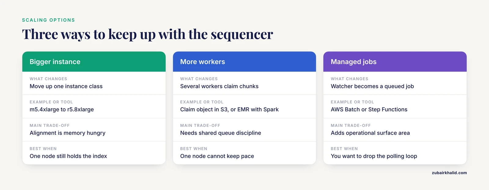
When one worker cannot keep up with the sequencer, you have three escalation paths, in order of effort:

1. Bigger instance. Move from m5.4xlarge to r5.8xlarge (32 vCPU, 256 GB RAM). Alignment is memory hungry for large references, and bwa-mem2 indexes load fully into RAM.
2. Horizontal parallelism. Run several workers, each claiming chunks by writing its ID to a claim object in S3 before processing. Amazon EMR with Spark is the managed version of this idea. Flint's design demonstrates that a Spark cluster on EMR can absorb large reference collections and streaming read input while keeping per-sample latency under a minute at cluster scale [1], and Spark's built-in parallelism and streaming engine are what make that possible [1].
3. Managed orchestration. Replace the watcher with AWS Batch or Step Functions so that chunk processing is a queued job rather than a polling loop. This adds operational surface area but removes the fragile parts of the watcher script.

For the cluster path, the capacity inequality from Step 5 applies per node. Chunks per minute produced by the sequencer must stay below chunks per minute the cluster can process, with headroom for Spot interruptions.

Real-Time Variant Calling AWS Pipeline Tips

These tips come from the parts of the design where small choices have large consequences.

Size chunks so calling is stable, not just fast. A one million read pair chunk is a reasonable starting point for Illumina data. Smaller chunks reduce latency but increase the fraction of variants near chunk boundaries, where per-chunk evidence is incomplete. Larger chunks do the opposite. Pick the largest chunk that still meets your latency requirement, and record the choice in your run documentation.

Keep the reference immutable and versioned. Copy the reference and all index files into an S3 prefix identified by build and version. Never overwrite a reference in place. Every VCF should be traceable to a reference version, and the cheapest way to guarantee that is to treat the reference as write-once data.

Watch the watcher. The polling loop in Step 6 is deliberately simple. Add a heartbeat file (for example, touch a timestamp file after each successful chunk) and alert when it goes stale. A silently dead watcher looks identical to a slow sequencer until someone notices the merged VCF stopped updating.

Use S3 multipart uploads for large BAMs. Files over a few hundred megabytes should upload with aws s3 cp, which uses multipart automatically, rather than with hand-rolled curl PUTs that time out. A truncated BAM fails much later with EOF marker is absent, long after you have forgotten the upload.

Pre-warm indexes. bwa-mem2 loads its index into RAM at startup. If your watcher restarts per chunk, you pay index load time every time. Keep the watcher process resident and the aligner index hot in memory.

Log the full command line into the VCF header. bcftools writes the calling command into the header automatically. Preserve it. Six months from now, that header line is the only record of exactly how a call set was produced.

Budget for Spot with a fallback. Spot instances cut compute costs substantially, but a two-minute interruption warning is not enough time to finish a chunk. Design the chunk processor so an interrupted chunk is simply retried from scratch, which is cheap when chunks are small, and keep an on-demand fallback instance for the tail of a critical run.

Common Mistakes and Limitations

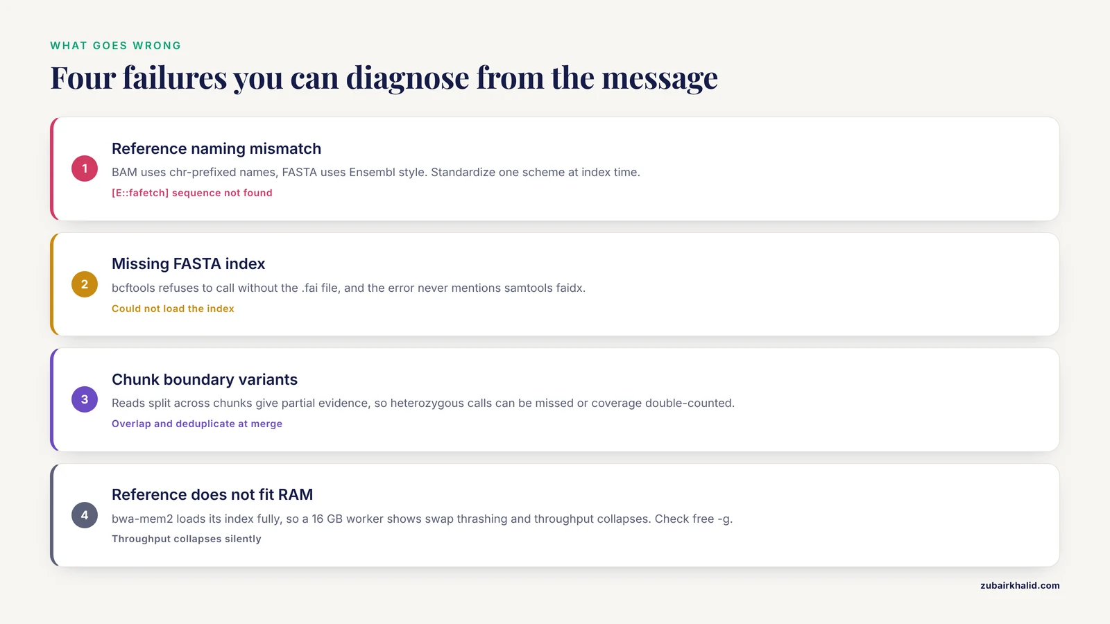
The following mistakes account for most of the pain in real deployments. Each one produces a specific, diagnosable failure.

Mismatched reference build. Aligning reads with one build and calling against another, or against a reference whose names differ from the alignment's @SQ lines, fails or silently misbehaves. The error [E::fafetch] The sequence "chr1" not found in the reference means your BAM uses one naming convention (chr-prefixed) and your FASTA uses another (Ensembl style, no prefix). Fix it by standardizing on one naming scheme everywhere, at index time.

Missing reference indexes. Running bcftools against a FASTA without a .fai file produces an index-loading error that does not mention samtools faidx. Whenever a tool complains it cannot open or load the reference, list the reference directory first and check for the .fai, plus the aligner index files.

Chunk boundary variants. A variant is called from the pileup of reads covering a position. Reads that overlap a chunk boundary exist in two chunks, each with partial evidence. Per-chunk calling can miss a heterozygous variant whose supporting reads are split across chunks, and can double-count coverage for variants in the overlap. The mitigations are overlapping chunks with deduplication at merge time, or periodically re-calling from the accumulated BAM over the full covered region. For clinical grade final calls, run one batch call over the complete run data and use the streaming call set only as the live preview. Be explicit with consumers about which file is which.

Treating per-chunk quality as final quality. Variant quality scores from a chunk with one million reads reflect one million reads of evidence. A position with 15x coverage in chunk 3 may have 60x coverage by chunk 9. Filters tuned on early chunks will be wrong later. Filter the merged call set, not the per-chunk ones.

Ignorable Spot interruptions that are not ignored. If a Spot interruption kills the worker mid-chunk and the chunk was never marked done, the watcher retries it, which is correct. If your done-marking happens before the S3 upload completes, the chunk is lost forever. Mark done only after uploads are confirmed.

One giant instance instead of many small ones. Alignment scales well across threads up to a point, then flatten. Ten m5.xlarge instances processing ten chunks concurrently often beats one instance processing ten chunks serially, and costs less, because per-chunk sort and call phases parallelize poorly at high thread counts on single nodes.

Forgetting that the reference must fit in RAM. bwa-mem2's index for a human genome occupies tens of gigabytes. A worker with 16 GB of RAM cannot hold it. This failure mode appears as swap thrashing, where the instance does not crash but throughput collapses. Check free -g if a run that took two minutes yesterday takes an hour today.

Confusing metagenomic profiling with variant calling. The published streaming systems in genomics, including Flint on EMR [1], profile reads against large collections of reference genomes. If your actual question is "which organisms are in this sample," a profiling pipeline against a large reference collection is the right tool, and Flint's design directly applies [1]. If your question is "which variants does this sample carry relative to one reference," the per-sample alignment and calling design in this article is the right tool. Building the wrong one for the question is the most expensive mistake of all.

No test genome in the loop. Every production change should be validated by running a known test sample through the new configuration and confirming the call set matches the previous configuration or a truth set. Teams that skip this discover reference naming problems in production data instead.

One limitation deserves a plain statement. Individual variant interpretation, whether in a clinical or veterinary context, requires a qualified professional. This pipeline produces call sets. It does not produce diagnoses.

Frequently Asked Questions

How fast is a real-time variant calling aws pipeline compared to batch processing?

A real-time pipeline produces its first variant calls within one chunk interval after the first reads arrive, often minutes, while batch processing waits for the entire run to finish. Published streaming work on AWS shows the approach scales well. Flint profiled one million Illumina paired-end reads against a 170 GB reference collection on 64 machines in 67 seconds [1]. Your per-chunk latency depends on chunk size, thread count, and reference size, so measure it on your own data rather than assuming any published figure transfers.

Can I run this pipeline on Amazon EMR with Spark instead of EC2?

Yes. Spark on EMR is the right choice when your reference collection is too large for one node or when you want managed cluster scaling. Flint demonstrates the pattern directly, running on Amazon's Elastic MapReduce service and using Spark's parallelism and streaming engine to map reads against a very large collection of genomes in near real time [1]. For single-reference, single-sample variant calling, a single EC2 worker is simpler and usually sufficient.

How do I choose the chunk size for streaming reads?

Choose the largest chunk size whose processing time stays comfortably below the time the sequencer needs to produce the next chunk, then verify that chunk-boundary variant loss is acceptable at that size. One million read pairs per chunk is a practical starting point for Illumina data. If a chunk takes longer to process than the inter-chunk interval, you fall behind and the merged VCF ages, which defeats the purpose of streaming.

Do I need GATK for variant calling on AWS?

No. bcftools handles SNP and indel calling well for many workflows, and it pipes cleanly for streaming designs. GATK adds joint calling, sophisticated recalibration, and a broad ecosystem of established best-practice steps, which matter for human clinical work. For bacterial genomes and for a first real-time system, bcftools keeps the toolchain small and the pipeline debuggable.

What does this cost to run?

Costs depend on instance type, run duration, and data transfer, and no source in the genomic literature fixes those numbers for your configuration. The dominant cost is compute time, which you control through instance size, Spot usage, and terminating instances when runs end. The E. coli test loop in this article runs on a small fraction of the compute of a human genome run, so validate your design there before scaling up.

How do I validate that my pipeline calls variants correctly?

Run a sample with a known truth set through the pipeline and compare. For human data, the Genome in a Bottle samples are the standard truth resources. For your E. coli smoke test, confirm a high mapping rate with samtools flagstat, spot-check calls against the reference annotation, and verify that repeated chunks produce consistent calls. Validation belongs in your continuous workflow, not just at initial setup.

Can this design handle nanopore or other long-read data?

The streaming architecture transfers directly, but the tools do not. bwa-mem2 and bcftools mpileup are tuned for short Illumina reads. Long-read calling uses different aligners and callers designed for noisy long reads, so you swap the align and call stages while keeping the chunked streaming skeleton, the S3 landing pattern, and the merge logic unchanged.

How many samples can one pipeline process at once?

As many as your cluster can process in parallel, one chunk at a time. Each sample is an independent chunk stream, so a fleet of workers behind a shared queue scales roughly linearly with node count until the reference index memory or S3 throughput becomes the limit. For very large reference collections, the Spark on EMR approach with its built-in parallelism is the published, demonstrated path to scale [1].

Sources

1. Large scale microbiome profiling in the cloud.